1-bit Stochastic Gradient Descent (1-bit SGD)
1-bit Stochastic Gradient Descent is a technique from Microsoft Research aimed at increasing the data parallelism inherent in training deep neural networks. They describe the technique in the paper 1-Bit Stochastic Gradient Descent and Application to Data-Parallel Distributed Training of Speech DNNs.
They accelerate training neural networks with stochastic gradient descent by:
- splitting up the computation for each minibatch across many nodes in a distributed system.
- reducing the bandwidth requirements for communication between nodes by exchanging gradients (instead of model parameters) and quantizing those gradients all the way to just 1 bit.
- they add the quantization error from Step 2 into the next minibatch gradient before quantization.
1-bit Stochastic Gradient Descent is available is a technique in Microsoft’s Cognitive Toolkit (CNTK).
References
1x1 Convolution
A 1x1 convolution or a network in network is an architectural technique used in some convolutional neural networks.
The technique was first described in the paper Network In Network.
A 1x1 convolution is a convolutional layer where the filter is of dimension \(1 \times 1\).
The filter takes in a tensor of dimension \(n_h \times n_w \times n_c\), over the \(n_c\) values in the third dimension and outputting a \(n_h \times n_w\) matrix. Subsequently, an activation function (like ReLU) is applied to the output matrix.
If we have \(p\) \(1 \times 1\) filters, then the output of the layer is a tensor of dimension \(n_h \times n_w \times p\). This is useful if the number of channels \(n_c\) in the previous layer of the network has grown too large and needs to be altered to \(p\) channels.
The \(1 \times 1\) convolution technique was featured in paper introducing the Inception network architecture, titled Going Deeper With Convolutions.
References
Abscissa
Abscissa is an obscure term for referring to the horizontal axis (the x-axis) on a two-dimensional coordinate plane.
Abstractive sentence summarization
Abstractive sentence summarization refers to creating a shorter version of a sentence with the same meaning.
This is in contrast to extractive sentence summarization, which pulls the most informative sentences from a document.
Related Terms
ACCAMS
ACCAMS: Additive Co-Clustering to Approximate Matrices Succinctly
Related Terms
References
Activation function
In neural networks, an activation function defines the output of a neuron.
The activation function takes the dot product of the input to the neuron (\(\mathbf x\)) and the weights (\(\mathbf w\)).
Typically activation functions are nonlinear, as that allows the network to approximate a wider variety of functions.
Related Terms
References
- Activation function - Wikipedia
(en.wikipedia.org) - Commonly used activation functions - Stanford CS231n notes
(cs231n.github.io)
AdaBoost
AdaBoost, short for Adaptive Boosting, aka Weight Boosted Trees, uses the same training set over and over. Increases the margin (separation) like SVMs.
ADADELTA
ADADELTA is a gradient descent-based optimization algorithm. Like AdaGrad, ADADELTA automatically tunes the learning rate.
References
AdaGrad
AdaGrad is a gradient-descent based optimization algorithm. It automatically tunes the learning rate based on its observations of the data’s geometry. AdaGrad is designed to perform well with datasets that have infrequently-occurring features.
Related Terms
References
- Adaptive Subgradient Methods for Online Learning and Stochastic Optimization
(jmlr.org) - An overview of gradient descent optimization algorithms - Sebiastian Ruder
(sebastianruder.com)
ADAM Optimizer
ADAM, or Adaptive Moment Estimation, is a stochastic optimization method introduced by Diederik P. Kingma and Jimmy Lei Ba.
They intended to combine the advantages of Adagrad’s handling of sparse gradients and RMSProp’s handling of non-stationary environments.
Related Terms
References
- Adam: A Method for Stochastic Optimization
(arxiv.org) - ADAM - An overview of gradient descent optimization algorithms - Sebastian Ruder
(sebastianruder.com)
Adaptive learning rate
The term adaptive learning rate refers to variants of stochastic gradient descent with learning rates that change over the course of the algorithm’s execution.
Allowing the learning rate to change dynamically eliminates the need to pick a “good” static learning rate, and can lead to faster training and a trained model with better performance.
Some adaptive learning rate algorithms are: - Adagrad - ADADELTA - ADAM
Additive clustering
Additive model
Related Terms
References
Adversarial autoencoder
Related Terms
References
Adversarial Variational Bayes
References
Affine space
Related Terms
Affinity analysis
Related Terms
References
Affinity propagation clustering
References
AlexNet
AlexNet is a convolutional neural network architecture proposed by Alex Krizhevsky, Ilya Sutskever, and Geoffrey Hinton in 2012.
At the time, it achieved state-of-the-art performance on the test set for the 2010 ImageNet Large Scale Visual Recognition Competition (LSVRC). A variant of the model won the 2012 ImageNet LSVRC with a top-5 test error rate of 15.3%–ten percentage points ahead of the second place winner.
Related Terms
References
Alternating conditional expectation (ACE) algorithm
References
Anchor box
Anchor boxes are a technique used in some computer vision object detection algorithms to help identify objects of different shapes.
Anchor boxes are hand-picked boxes of different height/width ratios (for 2-dimensional boxes) designed to match the relative ratios of the object classes being detected. For example, an object detector that detects cars and people may have a wide anchor box to detect cars and a tall, narrow box to detect people.
The Fast R-CNN paper introduced the idea of using the \(k\)-means-clustering to automatically determine the appropriate anchor box dimensions for a given \(k\) number of anchor boxes.
References
Antonym
Association rule mining
Related Terms
References
- Association rule learning - Wikipedia
(en.wikipedia.org) - Mining association rules between sets of items in large databases
(dl.acm.org)
Attention Mechanism
Related Terms
Autocorrelation matrix
References
Autoencoder
Autoencoders are an unsupervised learning model that aim to learn distributed representations of data.
Typically an autoencoder is a neural network trained to predict its own input data. A large enough network will simply memorize the training set, but there are a few things that can be done to generate useful distributed representations of input data, including:
- constraining the size of the model, forcing it to learn a lower-dimensional representation that can be used to re-construct the original higher-dimensional data points.
- adding artificial noise to the initial data points, and training the autoencoder to predict the data points minus the artificial noise. See denoising autoencoder for more information.
Related Terms
- Adversarial autoencoder
- Adversarial Variational Bayes
- Contractive autoencoder (CAE)
- Denoising autoencoder
- Self-supervised learning
- Semantic hashing
- Stacked autoencoder
- Variational Autoencoder (VAE)
References
- Autoencoder - Wikipedia
(en.wikipedia.org) - Autoencoders - Deep Learning Tutorial
(deeplearning.net) - What is the difference between an autoencoder and a neural network?
(www.quora.com)
Average pooling
Backprop
See Backpropagation.Backpropagation Through Time (BPTT)
References
Backpropagation
A technique to find good weight values in a neural network by trying different weights, and seeing if the change contributes positively to prediction quality.
Synonyms
- Backprop
Related Terms
- 1-bit Stochastic Gradient Descent (1-bit SGD)
- Backpropagation Through Time (BPTT)
- Long Short-Term Memory (LSTM)
References
- Yes you should understand backprop - Andrej Karpathy
(medium.com) - Backpropagation - Wikipedia
(en.wikipedia.org)
Bag-of-n-grams
A bag-of-\(n\)-grams model is a way to represent a document, similar to a [bag-of-words][/terms/bag-of-words/] model.
A bag-of-\(n\)-grams model represents a text document as an unordered collection of its \(n\)-grams.
For example, let’s use the following phrase and divide it into bi-grams (\(n = 2\)).
James is the best person ever.
becomes
<start>JamesJames isis thethe bestbest personperson ever.ever.<end>
In a typical bag-of-\(n\)-grams model, these 6 bigrams would be a sample from a large number of bigrams observed in a corpus. And then James is the best person ever. would be encoded in a representation showing which of the corpus’s bigrams were observed in the sentence.
A bag-of-\(n\)-grams model has the simplicity of the bag-of-words model, but allows the preservation of more word locality information.
Bag-of-words
The phrase bag-of-words typically refers to a way of representing text in natural language processing, although it has been applied to computer vision.
A bag-of-words representation contains how many times each word appears in a document, but disregards the order of the words.
Often, bag-of-words models will only include the \(k\) most frequent words in a corpus. This reduces the memory needed to store relatively-infrequent words, and the underlying representation of the document is mostly the same because common words dominate the document.
Bag-of-words models are often highly effective at representing documents in tasks like classification, clustering, or topic modeling. But they can struggle with tasks where word order matters, like sentiment analysis and machine translation. For example, in a bag-of-words model, the phrase “dog bites man” and “man bites dog” have identical representations.
Related Terms
References
- Bag-of-words model - Wikipedia
(en.wikipedia.org) - Bag of Words Meets Bags of Popcorn - Kaggle
(www.kaggle.com)
Bagging
Bagging, short for bootstrap aggregating, is training different base learners on different subsets of the training set randomly, by drawing random training sets from the given sample (with replacement).
References
Batch normalization
Batch normalization is a technique used to improve the stability and performance of deep neural networks. It works by normalizing the input data at each layer, which allows the network to learn more effectively. Batch normalization has been shown to improve training times, accuracy, and robustness of deep neural networks.
Related Terms
References
- Batch Normalization: Accelerating Deep Network Training by Reducing Internal Covariate Shift
(arxiv.org) - Batch Normalization — What the hey?
(gab41.lab41.org) - Why does batch normalization help? - Quora
(www.quora.com) - Understanding the backward pass through Batch Normalization Layer
(kratzert.github.io)
Bayesian optimization
Related Terms
Bayesian Probabilistic Matrix Factorization (BPMF)
Beam search
Beam search is a memory-restricted version of breadth-first search.
Beam search commonly appears in machine translation or other literature where sequence-to-sequence learning is common. In this domain, beam search allows the neural network to consider many candidate responses instead of selecting the highest-scoring token at each step.
Google’s blog post announcing SyntaxNet explains the advantages of beam search for sequence-to-sequence learning in greater detail: > At each point in processing many decisions may be possible—due to ambiguity—and a neural network gives scores for competing decisions based on their plausibility. For this reason, it is very important to use beam search in the model. Instead of simply taking the first-best decision at each point, multiple partial hypotheses are kept at each step, with hypotheses only being discarded when there are several other higher-ranked hypotheses under consideration.
References
- Beam search - Wikipedia
(en.wikipedia.org) - Why is beam search required in sequence-to-sequence transduction using recurrent neural networks? - Quora
(www.quora.com)
Bias-variance tradeoff
The bias-variance tradeoff refers to the problem of minimizing two different sources of error when training a supervised learning model:
Bias - Bias is a consistent error, possibly from the algorithm having made an incorrect assumption about the training data. Bias is often related to underfitting.
Variance - Variances comes from a high sensitivity to differences in training data. Variance is often related to overfitting.
It is typically difficult to simultaneously minimize bias and variance.
References
Bias
Related Terms
References
- Bias of an estimator - Wikipedia
(en.wikipedia.org) - Bias (statistics) - Wikipedia
(en.wikipedia.org)
Bidirectional LSTM
Related Terms
Bidirectional Recurrent Neural Network (BRNN)
Bilingual Evaluation Understudy (BLEU)
Related Terms
Binary Tree LSTM
References
Bit transparency (audio)
A digital audio system satisfies bit transparency if audio data can pass through the system without being changed.
A system can fail to be bit-transparent if it performs any type of digital signal processing–such as changing the audio’s sample rate. Some audio operations–like converting audio samples from integer to float and back–can either be bit-transparent or not depending on the implementation.
An audio system can be tested for bit-transparency by giving a random sequence of bits as input and testing that the output is bit-for-bit identical to the input.
References
Black-Box optimization
Related Terms
Boltzmann machine
References
Boosting
Learners trained serially so that instances on which the preceding base learners are not accurate are given more emphasis in training later base-learners; actively tries to generate complementary learners, instead of leaving this to chance.
References
Bounding box
A bounding box is a rectangle (in 2D datasets) or rectangular prism (in 3D datasets) drawn around an object identified in an image.
Object localization is a task in computer vision where a model is trained to draw bounding boxes around object detected in an image.
Related Terms
Burstiness
Wikipedia defines burstiness as follows:
In statistics, burstiness is the intermittent increases and decreases in activity or frequency of an event. One of measures of burstiness is the Fano factor—a ratio between the variance and mean of counts.
Word Burstiness
In natural language processing, burstiness has a slightly more specific definition, defined by Slava Katz in the mid 1990s.
The authors of Accounting for Burstiness in Topic Models give the following succinct definition of burstiness:
Church and Gale (1995) note that real texts systematically exhibit this phenomenon: a word is more likely to occur again in a document if it has already appeared in the document. Importantly, the burstiness of a word and its semantic content are positively correlated; words that are more informative are also more bursty.
Additionally, burstiness also tells us that later appearances of a word are less significant than the first appearance.
If a term is used once in a document, then it is likely to be used again. This phenomenon is called burstiness, and it implies that the second and later appearances of a word are less significant than the first appearance.
Related Terms
References
Capture-recapture model
A capture-recapture model is a technique to estimate an unknown population by capturing, tagging, and re-capturing samples from the population.
In the article How many Mechanical Turk workers are there?, Panos Ipeirotis explains a simple version of a capture-recapture model as follows:
The simplest possible technique is the following:
Capture/marking phase: Capture \(n_1\) animals, mark them, and release them back.
Recapture phase: A few days later, capture \(n_2\) animals. Assuming there are \(N\) animals overall, \(n_1/N\) of them are marked. So, for each of the \(n_2\) captured animals, the probability that the animal is marked is \(n_1/N\) (from the capture/marking phase).
Calculation: On expectation, we expect to see \(n_2 \cdot \frac{n_1}{N}\) marked animals in the recapture phase. (Notice that we do not know \(N\).) So, if we actually see \(m\) marked animals during the recapture phase, we set \(m = n_2 \cdot \frac{n_1}{N}\) and we get the estimate that:
\[N=n_1 \cdot \frac{n_2}{m}\]
He adds that this basic version of a capture-recapture model makes the following assumptions, and the estimate \(N\) can be inaccurate when these assumptions are violated:
Assumption of no arrivals / departures (“closed population”): The vanilla capture-recapture scheme assumes that there are no arrivals or departures of workers between the capture and recapture phase.
Assumption of no selection bias (“equal catchability”): The vanilla capture-recapture scheme assumes that every worker in the population is equally likely to be captured.
References
Catastrophic forgetting
Catastrophic forgetting (or catastrophic interference) is a problem in machine learning where a model forgets an existing learned pattern when learning a new one.
The model uses the same parameters to recognize both patterns, and learning the second pattern overwrites the parameters’ configuration from having learned the first pattern.
References
- Overcoming catastrophic forgetting in neural networks
(arxiv.org) - Catastrophic interference - Wikipedia
(en.wikipedia.org) - Catastrophic forgetting - Standout Publishing
(standoutpublishing.com) - Catastrophic Interference in Connectionist Networks: The Sequential Learning Problem
(www.sciencedirect.com)
Categorical mixture model
Child-Sum Tree-LSTM
References
Chinese Restaurant Process
Related Terms
Chunking
The paper Natural Language Processing (almost) from Scratch describes chunking as:
Also called shallow parsing, chunking aims at labeling segments of a sentence with syntactic constituents such as noun or verb phrases (NP or VP). Each word is assigned only one unique tag, often encoded as a begin-chunk (e.g., B-NP) or inside-chunk tag (e.g., I-NP).
Clustering stability
Related Terms
Clustering
Related Terms
- Additive clustering
- Affinity propagation clustering
- Clustering stability
- Co-clustering
- Community structure
- K-Means clustering
- Nonparametric clustering
- Parametric clustering
- Unsupervised learning
Co-adaptation
In neural networks, co-adaptation refers to when different hidden units in a neural networks have highly correlated behavior.
It is better for computational efficiency and the the model’s ability to learn a general representation if hidden units can detect features independently of each other.
A few different regularization techniques aim at reducing co-adapatation–dropout being a notable one.
References
Co-clustering
Related Terms
Codebook collapse
Codebook collapse is a problem that arises when training generative machine learning models that generate outputs using a fixed-length codebook, such as the Vector-Quantized Variational Autoencoder (VQ-VAE).
In ideal scenarios, the model’s fixed-size codebook is large enough to create a diverse set of output values. Codebook collapse happens when the model only learns to use a few of the values in the codebook–artificially limiting the diversity of outputs that the model can generate.
Codebook collapse is analogous to mode collapse, another problem commonly faced when training generative models.
Related Terms
Codebook
A codebook is a fixed-size table of embedding vectors learned by a generative model such as a vector-quantized variational autoencoder (VQ-VAE).
Generative models typically encode inputs into \(n\)-dimensional embedding vectors (for some \(n\)) in a continuous vector space of dimension \(\mathbb R^n\). Then, these generative models learn to decode these embedding vectors into a desired output.
Generative models that use a codebook–like the VQ-VAE–discretize embedding vectors by outputting the closest vector in the codebook. This restricts the potential number of outputs if the model only emits a single codebook value, but by having the model emit a sequence vectors from the codebook, it is possible for a small codebook to generate an enormous number of possible values.
Models like the VQ-VAE also learn the codebook values via gradient descent–just like how the model’s encoder and decoder are learned via gradient descent.
Related Terms
References
Collaborative filtering
Related Terms
Collaborative Topic Regression (CTR)
Community detection
Community detection refers to the problem of detecting whether a graph has community structure.
Community structure
Related Terms
References
Computer vision
Computer vision is the field of teaching computers to perceive sensor data–such as from cameras, RADAR, and LIDAR sensors–to achieve an understanding of what is in the data.
Computer vision is a wide-ranging field that comprises of many techniques and subfields.
Related Terms
- Anchor box
- Neural style transfer
- Non-max suppression
- Object detection
- Object localization
- YOLO (object detection algorithm)
References
Conditional GAN
Conditional Markov Models (CMMs)
Conditional Random Fields (CRFs)
References
Confusion matrix
Connectionism
References
Connectionist Temporal Classification (CTC)
Connectionist Temporal Classification is a term coined in a paper by Graves et al. titled Connectionist Temporal Classification: Labelling Unsegmented Sequence Data with Recurrent Neural Networks.
It refers to the use of recurrent neural networks (which is a form of connectionism) for the purpose of labeling unsegmented data sequences (AKA temporal classification).
References
Constituency Tree-LSTM
References
Contextual Bandit
References
- Contextual Bandit - Multi-armed Bandit - Wikipedia
(en.wikipedia.org) - An Introduction to Contextual Bandits - Stream
(getstream.io)
Continuous-Bag-of-Words (CBOW)
Continuous Bag of Words refers to a algorithm that predicts a target word from its surrounding context.
CBOW is one of the algorithms used for training word2vec vectors.
Related Terms
Contractive autoencoder (CAE)
Convex combination
A convex combination is a linear combination, where all the coefficients are greater than 0 and sum to 1.
The Convex combination Wikipedia article gives the following example:
Given a finite number of points \(x_1, x_2, \ldots, x_n\) in a real vector space, a convex combination of these points is a point of the form
\[ a_1 x_1 + a_2 x _2 + \ldots + a_n x_n \] is a convex combination if all real numbers \(a_i \geq 0\) and \(a_1 + a_2 + \ldots + a_n = 1\)
Related Terms
References
Convex hull
The convex hull of a set \(X\) in an affine space over the reals is the smallest convex set that contains \(X\). When the points are two dimensional, the convex hull can be thought of as the rubber band around the points of \(X\).
As per Wikipedia, a convex set is the smallest affine space closed under convex combination.
A convex combination is a linear combination where all the coefficients are greater than 0 and all sum to 1.
Related Terms
References
- Convex hull - Wikipedia
(en.wikipedia.org) - Convex set - Wikipedia
(en.wikipedia.org) - Convex combination - Wikipedia
(en.wikipedia.org)
Convex optimization
Related Terms
Convolution
Convolution is an operation where a filter (a small matrix) is applied to some input (typically a much larger matrix).
Convolution is a common operation in image processing, but convolution has also found some applications in natural language processing, audio processing, and other fields of machine learning.
Padding
Padding is a preprocessing step before a convolution operation. The input matrix is often padded to control the output dimensions of the convolution, or ot preserve information around the edges of the input matrix.
Stride
Stride is the number of steps the filter takes in the convolution operation.
Calculating the output dimensions of a convolution
For example, let’s say we have \(n \times n\) matrix \(A\) and a \(f \times f\) filter \(F\). The output dimension depends on two parameters – padding \(p\) and stride \(s\).
The dimensions for the output matrix \(A * F\) will be
\[ \left \lfloor \frac{n + 2p - f}{s} + 1 \right \rfloor \times \left \lfloor \frac{n + 2p - f}{s} + 1 \right \rfloor \].
In a same convolution, \(s = 1\) and \(p = \frac{f - 1}{2}\). The \(n \times n\) matrix \(A\) gets padded to $ n + p n + p$ and the output matrix becomes \(n \times n\).
Related Terms
- 1x1 Convolution
- Convolutional Neural Networks (CNN)
- Narrow convolution
- One-dimensional convolution
- Padding (convolution)
- Same convolution
- Sobel filter (convolution)
- Stride (convolution)
- Valid convolution
- Wide convolution
Convolutional Neural Networks (CNN)
Related Terms
- 1x1 Convolution
- AlexNet
- Anchor box
- Deep Convolutional Generative Adversarial Network (DCGAN)
- Dynamic k-Max Pooling
- Fast R-CNN
- GoogLeNet
- Inception
- Inceptionism
- k-Max Pooling
- LeNet
- Narrow convolution
- Neural style transfer
- Padding (convolution)
- Pooling layer
- R-CNN
- ResNet
- Same convolution
- Sobel filter (convolution)
- Stride (convolution)
- Valid convolution
- VGGNet
- Wide convolution
- YOLO (object detection algorithm)
- YOLOv2 (object detection algorithm)
- Zero padding
References
- Convolutional neural network - Wikipedia
(en.wikipedia.org) - Stanford CS231n Convolutional Neural Networks for Visual Recognition
(cs231n.github.io) - Understanding convolutional neural networks for NLP - WildML
(www.wildml.com)
Coreference resolution
The Stanford NLP group defines coreference resolution as:
Coreference resolution is the task of finding all expressions that refer to the same entity in a text. It is an important step for a lot of higher level NLP tasks that involve natural language understanding such as document summarization, question answering, and information extraction.
Coreference resolution should not be confused with Named Entity Recognition, which is focused on labeling sequences of text that refer to entities–but not focused on linking those entities together.
Related Terms
Cosine similarity
Covariance
Covariate shift
Related Terms
References
Cross-Entropy loss
Cross validation
Cross-validation refers to a group of techniques for dividing a dataset into multiple pieces.
Many methods of cross validation boil down to some variation of the following steps:
- Split the input dataset into a training dataset and a validation dataset.
- Train a model on the training dataset.
- Measure the trained model’s accuracy against the validation set.
- Repeat the above steps with different training/validation splits, allowing you to measure the variance in validation accuracy caused by different splits.
For example, \(k\)-fold cross validation is a more general version of the above procedure:
- The input dataset is divided into \(k\) shards.
- Each individual shard is used as a separate validation dataset, measuring the performance of a model trained against the other \(k-1\) shards.
Related Terms
References
- Cross-validation (statistics)
(en.wikipedia.org) - A Gentle Introduction to k-fold Cross-Validation
(machinelearningmastery.com)
Data augmentation
Data augmentation is the process of using computer algorthms or other synthetic means to increase the size of a collected dataset.
Machine learning algorithms typically become more resistant to overfitting when they are trained with more data. But in many cases, it can be expensive to collect more data.
It is often possible to significantly increase the size of a dataset by computing simple transformations that are unlikely to be learned by the model, but also do not change the value of the labels.
For example, if one were building a model to identify pictures of cats versus non-cats, flipping the pictures horizontally or vertically increases the size of the available image data. When the pictures are flipped, whether they contain a cat or not doesn’t change. Despite this, many statistical models would be unlikely to learn flip-invariance without a significant amount of data–either collected from the real-world or generated through data augmentation.
Related Terms
References
- Data Augmentation - Convolutional Neural Networks - deeplearning.ai
(www.coursera.org) - Understanding data augmentation for classification: when to warp?
(arxiv.org) - What you need to know about data augmentation for machine learning - Cartesian Faith
(cartesianfaith.com)
Data parallelism
Data parallelism is when data is distributed across multiple nodes in a distributed computing environment, and then each node acts on the data in parallel.
On each node, the computation is the same, but the data is different.
Related Terms
References
- Data parallelism - Wikipedia
(en.wikipedia.org) - What is the difference between model parallelism and data parallelism? - Quora
(www.quora.com)
Decision tree
A supervised learning method that iteratively refines a prediction by asking questions about the input feature most likely to affect the outcome, making a ‘tree’ of question branches.
Related Terms
References
Deep Convolutional Generative Adversarial Network (DCGAN)
DCGAN refers to a model described by Radford, Metz, and Chintala that uses deep convolutional neural networks in a generative adversarial network model.
Generative adversarial networks (GANs) are structured as a competition between two models:
- a generative model that tries to create fake examples of training data interspersed with real training data.
- a discriminative model that tries to classify real examples from fake ones.
DCGAN uses deep convolutional neural networks for both models. Convolutional neural networks (CNNs) are well-known for their performance on image data. DCGAN uses the strong performance of (CNNs) to learn unsupervised representations of the input data.
References
Deep Learning
Deep Learning is about learning using neural networks with multiple [hidden layers][2].
References
Denoising autoencoder
Dependency Tree LSTM
References
Derivative-free optimization
References
- Derivative-free optimization - Wikipedia
(en.wikipedia.org) - Derivative-free optimization: A review of algorithms and comparison of software implementations
(thales.cheme.cmu.edu)
Differential Evolution (DE)
Related Terms
References
Differential Topic Modeling
Dimensionality reduction
Dimensionality reduction is about taking a set of data, and reducing its number of dimensions in such a way as to balance information size and independence of the features’ information. The point is to get a smaller dataset that still retains most of the original information.
References
Dirichlet-multinomial distribution
References
Dirichlet process
Distance metric learning
Distance metric learning is the task of using a labeled dataset to learn a similarity learning where the similarity function has to obey the four axioms of a distance metric.
The problem is typically defined with a dataset where there some of the datapoints are known to be “similar” and should be closer to each other than another arbitrarily-chosen datapoint in the dataset.
Distance metric learning first received significant attention in the machine learning community from the 2002 NIPS paper titled Distance metric learning, with application to clustering with side-information.
Axioms of a distance metric
The four axioms of a distance metric are:
- Non-negativity: \(d(x, y) \geq 0\) – The distance must always be greater than zero.
- Identity of indiscernibles: \(d(x, y) = 0 \Leftrightarrow x = y\) – The distance must be zero for two elements that are the same (i.e. indiscernible from each other).
- Symmetry: \(d(x,y) = d(y,x)\) – The distances must be the same, no matter which order the parameters are given.
- Triangle inequality: \(d(x,z) \leq d(x,y) + d(y,z)\) – For three elements in the set, the sum of the distances for any two pairs must be greater than the distance for the remaining pair.
Related Terms
References
- Distance Metric Learning: A Comprehensive Survey
(www.cs.cmu.edu) - Distance metric learning, with application to clustering with side-information
(ai.stanford.edu)
Distance metric
As per Wikipedia, a distance metric, metric, or distance function, “is a function that defines a distance between each pair of elements of a set.”
A distance metric \(d(\cdot)\) requires the following four axioms to be true for all elements \(x\), \(y\), and \(z\) in a given set.
- Non-negativity: \(d(x, y) \geq 0\) – The distance must always be greater than zero.
- Identity of indiscernibles: \(d(x, y) = 0 \Leftrightarrow x = y\) – The distance must be zero for two elements that are the same (i.e. indiscernible from each other).
- Symmetry: \(d(x,y) = d(y,x)\) – The distances must be the same, no matter which order the parameters are given.
- Triangle inequality: \(d(x,z) \leq d(x,y) + d(y,z)\) – For three elements in the set, the sum of the distances for any two pairs must be greater than the distance for the remaining pair.
Related Terms
References
Distributed representation
In machine learning, data with a local representation typically has 1 unit per element. A 5-word vocabulary might be defined by a 5-dimensional vector, with \([1, 0, 0, 0, 0]^T\) denoting the first word, \([0, 1, 0, 0, 0]^T\) denoting the second word, and so forth.
Distributed representations are the opposite, instead of concentrating the meaning of a data point into one component or one “element”, the meaning of the data is distributed across the whole vector.
The word that is \([1, 0, 0, 0, 0]^T\) in a local representation might look like \([-0.150, -0.024, -0.233, -0.253, -0.183]^T\) in a distributed representation.
Related Terms
References
- Distributed Representation - Directory of Cognitive Science
(www.bcp.psych.ualberta.ca) - Local and distributed representations - Programming Methods for Cognitive Science
(www.indiana.edu)
Distributional similarity
Distributional similarity is the idea that the meaning of words can be understood from their context.
This should not be confused with the term distributed representation, which refers to the idea of representing information with relatively dense vectors as opposed to a one-hot representation.
References
- Distributional semantics - Wikipedia
(en.wikipedia.org) - word2vec - Stanford CS224N Lecture 2
(www.youtube.com)
doc2vec
doc2vec is the gensim library’s name for its paragraph vector implementation. doc2vec can be used to generate unsupervised representations of sentences, paragraphs, and documents.
Related Terms
Domain adaptation
References
Dropout
Dropout or dilution is a technique for regularizing neural networks, developed by Hinton et al. and published in the paper Improving neural networks by preventing co-adaptation of feature detectors.
The core idea behind dropout is to randomly set some of the weights in a neural network to \(0\) during the training phase.
Dropout add a hyperparameter of a “keep probability”. This is the probability that a weight value is left undisturbed– that it will not be set to \(0\).
Dropout can be considered analogous to model-averaging because the process simulates training many similar neural networks on the same data.
Related Terms
References
- Dilution (neural networks) - Wikipedia
(en.wikipedia.org) - How does the dropout method work in deep learning? - Quora
(www.quora.com) - Improving neural networks by preventing co-adaptation of feature detectors
(arxiv.org)
Dying ReLU
Dying ReLU refers to a problem when training neural networks with rectified linear units (ReLU). The unit dies when it only outputs 0 for any given input.
When training with stochastic gradient descent, the unit is not likely to return to life, and the unit will no longer be useful during training.
Leaky ReLU is a variant that solves the Dying ReLU problem by returning a small value when the input \(x\) is less than 0.
References
Dynamic k-Max Pooling
Related Terms
References
Early stopping
Embed, Encode, Attend, Predict
The phrase Embed, Encode, Attend, Predict refers to Matthew Honnibal’s conceptual framework for deep learning for natural language processing.
The steps have the following meanings:
Embed – This is the process of turning text or sparse vectors into dense word embeddings. These embeddings are much easier to work with than other representations, and do an excellent job of capturing semantic information.
Encode – This is the process of encoding a sequence of word vectors into a matrix, using techniques like recurrent neural networks or LSTMs.
Attend – This refers to taking the matrix from the Encode step and transforming it into a vector, most likely using an attention mechanism.
Predict – The final step in the Natural Language Processing pipeline is making a prediction given the input text.
References
Entailment
The word entailment has many meanings. Please review Wikipedia’s disambiguation page for “entail” for definitions that do not refer to textual entailment.
Textual entailment refers to drawing a relation from an entailing text to an entailed hypothesis.
The Wikipedia page for textual entailment gives the following examples:
Textual entailment can be illustrated with examples of three different relations:
An example of a positive TE (text entails hypothesis) is:
- text: If you help the needy, God will reward you.
- hypothesis: Giving money to a poor man has good consequences.
An example of a negative TE (text contradicts hypothesis) is:
- text: If you help the needy, God will reward you.
- hypothesis: Giving money to a poor man has no consequences.
An example of a non-TE (text does not entail nor contradict) is:
- text: If you help the needy, God will reward you.
- hypothesis: Giving money to a poor man will make you a better person.
Synonyms
- Textual entailment
References
- Entailment (linguistics) - Wikipedia
(en.wikipedia.org) - Textual entailment - Wikipedia
(en.wikipedia.org) - A machine learning approach to textual entailment recognition
(disi.unitn.it) - Recognizing Textual Entailment
(l2r.cs.uiuc.edu)
Error-Correcting Tournaments
References
Expectation-maximization (EM) algorithm
References
Expectation
Related Terms
Exploding gradient problem
Related Terms
Exponential Linear Unit (ELU)
References
- Fast and Accurate Deep Network Learning by Exponential Linear Units (ELUs)
(arxiv.org) - Deep Residual Networks with Exponential Linear Unit
(arxiv.org)
Extractive sentence summarization
Extractive sentence summarization refers to programmatically creating a shorter version of a document by extracting the “important” parts.
TextRank is an example of an algorithm that can rank sentences in a document for the purpose of extractive summarization.
References
Face detection
Face detection is the problem of detecting wheter an image has a (usually human) face in it.
The problem of identifying whether the image has a specific single person’s face is called face verification. The problem of identifying whether the image has any of \(k\) person’s faces is called face recognition.
Related Terms
Face recognition
Face recognition is the problem of identifying whether an input image contains the faces of any of \(k\) people… or if the image has none of the \(k\) faces.
Face recognition is a harder problem than face verification because face verification only compares a single image to one person, whereas face recognition does this for \(k\) people.
Related Terms
References
Face verification
Face verification is the problem of identifying whether an image belongs to a person–given the one image and one person as the input.
Face verification is an easier problem than face recognition because face verification only compares a single image to one person, whereas face recognition does this for \(k\) people.
Related Terms
References
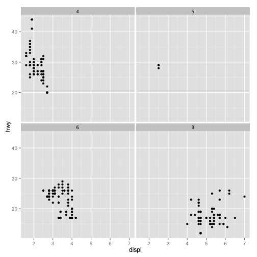
Facet
In statistical plotting, a facet is a type of plot. Data is split into subsets and the subsets are plotted in a row or grid of subplots.
The term is common among users of ggplot2, a plotting package for the R statistical computing language.
Facet is also the name of a plotting and visualizaton tool created by the People + AI Research (PAIR) initiative at Google.
References
Facet (disambiguation)
A facet can refer to a type of plot or chart designed to efficiently display multidimensional data.
Facets is also the name of a tool from Google’s People + AI Research (PAIR) lab designed to help explore datasets.
Facet (visualization tool)
Facets is a a plotting and visualizaton tool created by the People + AI Research (PAIR) initiative at Google.
Facets is broken into two tools with the following goals:
- Facets Overview – summarize statistics for features collected from datasets
- Facets Dive – explore the relationship between different features in a dataset
From the Facets homepage, they state that
Success stories of (Facets) Dive include the detection of classifier failure, identification of systematic errors, evaluating ground truth and potential new signals for ranking.
Related Terms
References
Fast Fourier transform (FFT)
References
Fast R-CNN
References
fastText
fastText is a project from Facebook Research for producing word embeddings and sentence classification.
The fastText project is hosted on Github and instructions for using their pre-trained word embeddings can be found here.
Feature learning
See Representation learning.Filter (convolution)
A filter (also known as a kernel) is a small matrix used in convolution operations.
Convolution filters are commonly used in image processing to modify images or extract features.
The dimensions of a convolution filter are typically small, odd, and square. For example, convolution filters are typically \(3 \times 3\) or \(5 \times 5\) matrices. Odd dimensions are preferred to even dimensions.
Synonyms
- Kernel (convolution)
Related Terms
References
Finite-state transducer (FST)
Related Terms
References
First-order information
First-order information is a term used to mean information obtained by computing the first derivative of a function. The first derivative of a function reveals the slope of a tangent line to the function. This gives a general idea of how the function is changing at that point, but does not give information about the curvature of the function–the second derivative is required for that.
First-order information should not be confused with first-order logic.
Related Terms
Gap statistic
References
Gaussian mixture model (GMM)
Related Terms
References
Generalized additive model (GAM)
References
Generative Adversarial Network (GAN)
A generative adversarial network (GAN) is a framework for training neural networks–often for the purpose of training neural networks to artificially generate novel data samples.
A GAN is structured as a game between two neural networks:
- a discriminator network that distinguishes between real-world data samples and artificially generated imitation data samples.
- a generator network that learns to create artificial data that is realistic enough to fool the discriminator.
A GAN is successfully trained when both of these goals are achieved:
- The generator can reliably generate data that fools the discriminator.
- The generator generates data samples that are as diverse as the distribution of the real-world data.
When the generator achieves both goals #1 and #2, it is theoretically capable of “perfect” artifiical data that no human or discriminative model could distinguish as fake.
However, in practice, there are many challenges to training a GAN to the point where the generator can produce realistic samples. For exmaple, many GANs suffer from mode collapse, where the generator network gets “stuck” generating only a few data samples.
Ian Goodfellow originally proposed GANs in a 2014 paper, originally formulating the GAN loss function as a two-player minimax game between the generator and discriminator. Since then, newer GAN variants have altered the loss function in other ways, such as using the Wasserstein loss function.
Related Terms
- Adversarial autoencoder
- Adversarial Variational Bayes
- Deep Convolutional Generative Adversarial Network (DCGAN)
- Minimax
- Mode collapse
- Neural style transfer
- Temporal Generative Adversarial Network (TGAN)
- Variational Autoencoder (VAE)
- Vector-Quantized Variational Autoencoders (VQ-VAE)
References
- Generative adversarial networks - Wikipedia
(en.wikipedia.org) - Generative adversarial networks
(arxiv.org) - NIPS 2016 tutorial: Generative Adversarial Networks
(arxiv.org)
Gibbs sampling
Related Terms
Global Average Pooling (GAP)
References
GloVe (Global Vectors) embeddings
GloVe, or Global Vectors, refers to a word embedding algorithm from the Stanford NLP group.
Related Terms
References
- GloVe: Global Vectors for Word Representation - Stanford NLP Group
(nlp.stanford.edu) - GloVe - Stanford NLP project page
(nlp.stanford.edu)
GoogLeNet
Related Terms
Gradient Clipping
References
- Gradient Clipping - Tensorflow Python Documentation
(www.tensorflow.org) - On the difficulty of training Recurrent Neural Networks
(arxiv.org)
Gradient descent
Gradient descent is an optimization algorithm designed to find the minimum of a function. Many machine learning algorithms use gradient descent or a variant.
Common variants include: - Stochastic Gradient Descent (SGD) - Minibatch Gradient Descent
Related Terms
Gradient
The gradient is the vector generalization of the derivative.
For a function \(f([x_1, \ldots, x_n]^T)\), the gradient \(\nabla_x f([x_1, \ldots, x_n]^T)\) is the vector containing the \(n\) partial derivatives of \(f\) with respect to each \(x_i\).
Related Terms
Gram matrix
Wolfram Mathworld defines Gram matrix as:
Given a set \(V\) of \(m\) vectors (points in \(\mathcal R^n\)), the Gram matrix \(G\) is the matrix of all possible inner products of \(V\), i.e., \[ g_{ij} = \mathbf v_i^T \mathbf v_j \]
References
- Gramian matrix - Wikipedia
(en.wikipedia.org) - Gram Matrix - Wolfram Mathworld
(mathworld.wolfram.com) - Gram matrix - Encyclopedia of Mathematics
(www.encyclopediaofmath.org)
Graph Neural Network
References
Graph
Related Terms
Grid search
Hadamard product
The Hadamard product refers to component-wise multiplication of the same dimension. The \(\odot\) symbol is commonly used as the Hadamard product operator.
Here is an example for the Hadamard product for a pair of \(3 \times 3\) matrices.
\[ \begin{bmatrix} a & b & c \\ d & e & f \\ g & h & i \end{bmatrix} \odot \begin{bmatrix} j & k & l \\ m & n & o \\ p & q & r \end{bmatrix} = \begin{bmatrix} aj & bk & cl \\ dm & ne & fo \\ gp & hq & ir \end{bmatrix} \]
Hamming distance
Harmonic Precision-Recall Mean (F1 Score)
The \(F_1\) score is a classification accuracy metric that combines precision and recall. It is designed to be useful metric when classifying between unbalanced classes or other cases when simpler metrics could be misleading.
When classifying between two cases (“positive” and “negative”), there are the four possible results of prediction:
| Actual Positive | Actual Negative | |
| Predicted Positive | True Positives | False Positives |
| Predicted Negative | False Negatives | True Negatives |
Precision answers the question, “What fraction of positive predictions are true predictions?”
A cancer diagnostic test that suggested that all patients have cancer would achieve
\[ \mathrm{Precision} = \frac{\mathrm{True\;Positives}}{\mathrm{True\;Positives} + \mathrm{False\;Positives}} \]
Recall answers the question, “Out of all the true positives, what fraction of them did we identify?”
A cancer diagnostic test that suggested that all patients have cancer would achieve perfect recall, as all patients that actually have cancer would be identified.
\[ \mathrm{Recall} = \frac{\mathrm{True\;Positives}}{\mathrm{True\;Positives + False\;Negatives}} \]
The F1 score is a way to combine precision and recall in the following way:
\[ F_1 = 2 * \frac{\mathrm{Precision} \times \mathrm{Recall}}{\mathrm{Precision} + \mathrm{Recall}} \]
For a classifier to have a high \(F_1\) score, it needs to have high precision and high recall.
References
He initialization
The term He initialization refers to the first author in the paper “Delving Deep into Rectifiers: Surpassing Human-Level Performance on ImageNet Classification”.
He initialization initializes the bias vectors of a neural network to \(0\) and the weights to random numbers drawn from a Gaussian distribution where the mean is \(0\) and the variance is \(\sqrt(2/n_l)\) where \(n_l\) is the dimension of the previous layer.
References
Helvetica scenario
See Mode collapse.Hessian-free optimization
Related Terms
References
- Hessian Free Optimization - Andrew Gibiansky
(andrew.gibiansky.com) - Deep learning via Hessian-free optimization
(www.cs.toronto.edu) - Hessian-free Optimization for Learning Deep Multidimensional Recurrent Neural Networks
(arxiv.org)
Hessian matrix
Related Terms
Hidden Markov Models (HMMs)
Hierarchical Dirichlet process (HDP)
Related Terms
Hierarchical Latent Dirichlet allocation (hLDA)
Hierarchical Softmax
Related Terms
Hinge loss
From the scikit-learn documentation, we get the following definition:
The hinge_loss function computes the average distance between the model and the data using hinge loss, a one-sided metric that considers only prediction errors. (Hinge loss is used in maximal margin classifiers such as support vector machines.)
Hopfield Network
A Hopfield network (HN) is a type of recurrent neural network(RNN). The HNs have only one layer, with each neuron connected to every other neuron: All neurons act as input and output. The model of the network consists of a set of neurons and corresponding set of unit delays, forming a multiple loop feedback system. The output of a neuron is, via a unit delay element, sent to all of the others neurons in the HN, except itself.
Some important properties of HNs are that all neurons have binary outputs (either 0, 1 or -1, 1), it isn’t allowed a connection from a neuron to itself, the neurons are updated at random order (asynchronously), and the weights between the neurons are symmetric. This last property guarantees that the energy function decreases while following the activation function rules, and HNs are guaranteed to converge to a local minimum.
Hopfield networks are used for pattern recognition, and provides a model for understanding human memory. A HN is initially trained to store a number of patterns, and then it’s able to recognize any of the learned patterns by exposure to only partial or even corrupted information about the pattern (it returns the closest pattern or the best guess). This property makes the Hopfield network a form of associative memory (or content-addressable memory). It’s applications include image detection and recognition, enhancement of X-Ray images, medical images restoration, etc.
Related Terms
References
Hypergraph
A hypergraph is a generalization of the graph. A graph has edges that connect pairs of vertices, but a hypergraph has hyperedges that can connect any number of vertices.
References
- Hypergraph - Wikipedia
(en.wikipedia.org) - Learning with Hypergraphs: Clustering, Classification, Embedding
(papers.nips.cc) - What are the applications of hypergraphs? - Math Overflow
(mathoverflow.net)
Hypernetwork
References
Hypernym
Related Terms
Hyperparameter
Related Terms
Hyponym
Related Terms
Identity mapping
Importance sampling
Imputation
Imputation means replacing missing data values with substitute values. There are several ways to do this such as choosing from a random distribution to avoid bias or by replacing the missing value with the mean or median of that column.
References
- 6 Different Ways to Compensate for Missing Values In a Dataset (Data Imputation with examples) - Will Badr
(towardsdatascience.com) - Imputation (statistics)
(en.wikipedia.org) - Defining, Analysing, and Implementing Imputation Techniques - Shashank Singhal
(scikit-learn.org)
Inception
Inception refers to a particular neural network model in the CVPR 2015 paper titled Going Deeper With Convolutions.
Related Terms
References
- google/inception - Github
(github.com) - Going Deeper With Convolutions
(arxiv.org) - Inceptionism: Going Deeper into Neural Networks
(research.googleblog.com) - How does the Inception module work in GoogLeNet deep architecture?
(www.quora.com) - Inception in Tensorflow - Github
(github.com) - Rethinking the Inception Architecture for Computer Vision
(arxiv.org) - Inception-v4, Inception-ResNet and the Impact of Residual Connections on Learning
(arxiv.org)
Inceptionism
Inceptionism refers to a visualization technique to understand what a neural network learned. The network is fed an image, asked what the network detected, and then that feature in the image is amplified. The full technique is described in the Google Research blog post titled Inceptionism: Going Deeper into Neural Networks.
Independent and Identically Distributed (i.i.d)
A collection of random variables is independent and identically distributed if they have these properties:
- they all have the same probability distribution.
- they are all mutually independent of each other.
Indian Buffet Process
References
Internal covariate shift
The term interal covariate shift comes from the paper Batch Normalization: Accelerating Deep Network Training by Reducing Internal Covariate Shift.
The authors’ precise definition is:
We define Internal Covariate Shift as the change in the distribution of network activations due to the change in network parameters during training.
In neural networks, the output of the first layer feeds into the second layer, the output of the second layer feeds into the third, and so on. When the parameters of a layer change, so does the distribution of inputs to subsequent layers.
These shifts in input distributions can be problematic for neural networks, especially deep neural networks that could have a large number of layers.
Batch normalization is a method intended to mitigate internal covariate shift for neural networks.
References
Inverted dropout
Inverted dropout is a variant of the original dropout technique developed by Hinton et al.
Just like traditional dropout, inverted dropout randomly keeps some weights and sets others to zero. This is known as the “keep probability” \(p\).
The one difference is that, during the training of a neural network, inverted dropout scales the activations by the inverse of the keep probability \(q = 1 - p\).
This prevents network’s activations from getting too large, and does not require any changes to the network during evaluation.
In contrast, traditional dropout requires scaling to be implemented during the test phase.
References
Jaccard index (intersection over union)
The Jaccard index–otherwise known as intersection over union–is used to calculate the similarity or difference of sample sets.
\[ J(\mathbb{A}, \mathbb{B}) = \frac{\left | \mathbb{A} \cap \mathbb{B} \right |} {\left | \mathbb{A} \cup \mathbb{B} \right |} \]
\[ 0 \leq J(\mathbb{A}, \mathbb{B}) \leq 1 \]
The index is defined to be 1 if the sets are empty.
Related Terms
Jacobian matrix
Related Terms
k-Max Pooling
Related Terms
References
K-Means clustering
Related Terms
Kernel (convolution)
See Filter (convolution).Kullback-Leibler (KL) divergence
Language segmentation
This phrase is most concisely described in in this work by David Alfter:
Language segmentation consists in finding the boundaries where one language ends and another language begins in a text written in more than one language. This is important for all natural language processing tasks.
[…]
One important point that has to be borne in mind is the difference between language identification and language segmentation. Language identification is concerned with recognizing the language at hand. It is possible to use language identification for language segmentation. Indeed, by identifying the languages in a text, the segmentation is implicitly obtained. Language segmentation on the other hand is only concerned with identifying language boundaries. No claims about the languages involved are made.
Laplacian matrix
Related Terms
Latent Dirichlet Allocation Differential Evolution (LDADE)
LDADE is a tool proposed by Agrawal et al. in a paper titled What is Wrong with Topic Modeling? (and How to Fix it Using Search-based Software Engineering).
It tunes LDA parameters using Differential Evolution to increase the clustering stability of standard LDA.
References
Latent Dirichlet allocation (LDA)
Related Terms
- Dirichlet process
- Hierarchical Dirichlet process (HDP)
- Hierarchical Latent Dirichlet allocation (hLDA)
- Latent Dirichlet Allocation Differential Evolution (LDADE)
- Latent Semantic Indexing (LSI)
- Pitman-Yor Topic Modeling (PYTM)
- Termite
Latent semantic analysis (LSA)
See Latent Semantic Indexing (LSI).Latent Semantic Indexing (LSI)
Synonyms
- Latent semantic analysis (LSA)
Related Terms
References
- Latent semantic indexing - Wikipedia
(en.wikipedia.org) - What is latent semantic indexing? - Search Engine Journal
(www.searchenginejournal.com) - Latent Semantic Indexing - Introduction to Information Retrieval
(nlp.stanford.edu)
Leaky ReLU
Leaky ReLU is a type of activation function that tries to solve the Dying ReLU problem.
A traditional rectified linear unit \(f(x)\) returns 0 when \(x \leq 0\). The Dying ReLU problem refers to when the unit gets stuck this way–always returning 0 for any input.
Leaky ReLU aims to fix this by returning a small, negative, non-zero value instead of 0, as such:
\[ f(x) = \begin{cases} \max(0,x) & x > 0 \\ \alpha x & x \leq 0 \end{cases} \] where \(\alpha\) is typically a small value like \(\alpha = 0.0001\).
Related Terms
Learning rate annealing
See Learning rate decay.Learning rate decay
Synonyms
- Learning rate annealing
Related Terms
References
- Decaying the learning rate - TensorFlow Documentation
(www.tensorflow.org) - Annealing the learning rate - Stanford CS231n
(cs231n.github.io)
Learning rate
Related Terms
Learning To Rank (LTR)
Learning-to-rank is the application of machine learning to ranking search results, recommendations, or similar information.
References
- Learning to rank - Wikipedia
(en.wikipedia.org) - Learning To Rank - Apache Solr Documentation
(cwiki.apache.org)
LeNet
LeNet was an early convolutional neural network proposed by Lecun et al in the paper Gradient-Based Learning Applied to Document Recognition.
LeNet was designed for handwriting recognition. Many modern convolutional neural network architectures are inspired by LeNet.
Related Terms
References
- Case Studies - Stanford CS231n Convolutional Neural Networks
(cs231n.github.io) - Gradient-Based Learning Applied to Document Recognition
(yann.lecun.com)
Lexeme
Likelihood
In statistics, likelihood is the hypothetical probability that a past event would yield a specific outcome. Probability is concerned with the future, but likelihood is concerned with the past.
Linear discriminant analysis (LDA)
Long Short-Term Memory (LSTM)
Long short term memory (LSTM) networks try to reduce the vanishing and exploding gradient problem during the backpropagation in recurrent neural networks. LSTM are in general, a RNN where each neuron has a memory cell and three gates: input, output and forget. The purpose of the memory cell is to retain information previously used by the RNN, or forget if needed. LSTMs are explicitly designed to avoid the long-term dependency problem in RNNs, and have been shown to be able to learn complex sequences better than simple RNNs.
The structure of a memory cell is: an input gate, that determines how much of information from the previous layer gets stored in the cell; the output gate, that determines how of the next layer gets to know about the state of the current cell; and the forget gate, which determines what to forget about the current state of the memory cell.
Related Terms
- Bidirectional LSTM
- Binary Tree LSTM
- Child-Sum Tree-LSTM
- Constituency Tree-LSTM
- Dependency Tree LSTM
- Gradient Clipping
- Multilayer LSTM
- N-ary Tree LSTM
- Peephole connection
- Sequence to Sequence Learning (seq2seq)
- Tree-LSTM
References
Loss function
Related Terms
Magnet loss
Magnet loss is a type of loss function used in distance metric learning machine learning problems. It was introduced in the paper Metric Learning with Adaptive Density Discrimination. The authors of the paper introduced magnet loss as an improvement over triplet loss and other loss functions designed to learn a distance metric.
Instead of working on individuals, pairs, or triplets of data points, magnet loss operates on entire regions of the embedding space that the data points inhabit. Magnet loss models the distributions of different classes in the embedding space and works to reduce the overlap between distributions.
References
- Metric Learning with Adaptive Density Discrimination
(arxiv.org) - Significance of Softmax-based Features in Comparison to Distance Metric Learning-based Features
(arxiv.org)
Margin
In machine learning, a margin often refers to the distance between the two hyperplanes that separate linearly-separable classes of data points.
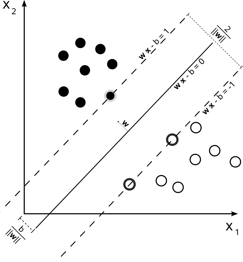
The term is most commonly used when discussing support vector machines, but often appears in other literature discussing boundaries between points in a vector space.
References
Market basket analysis
Markov Chain Monte Carlo (MCMC)
Related Terms
Max-margin loss
Max Pooling
Related Terms
Maximum A Posteriori (MAP) Estimation
Related Terms
Maximum Likelihood Estimation (MLE)
Related Terms
Maxout
References
Mean Reciprocal Rank (MRR)
\(\newcommand{\Correctrank}{\mathrm{rank}}\)
Mean Reciprocal Rank is a measure to evaluate systems that return a ranked list of answers to queries.
For a single query, the reciprocal rank is \(\frac 1 \Correctrank\) where \(\Correctrank\) is the position of the highest-ranked answer (\(1, 2, 3, \ldots, N\) for \(N\) answers returned in a query). If no correct answer was returned in the query, then the reciprocal rank is 0.
For multiple queries \(Q\), the Mean Reciprocal Rank is the mean of the \(Q\) reciprocal ranks.
\[\mathrm{MRR} = \frac 1 Q \sum_{i=1}^{Q} \frac 1 {\Correctrank_i}\]
References
- Chapter 14: Question Answering and Information Retrieval - Speech and Language Processing
(web.stanford.edu) - Mean reciprocal rank - Wikipedia
(en.wikipedia.org)
Mention-pair coreference model
References
Mention-ranking coreference model
Related Terms
References
Meronym
Meta learning
References
METEOR
METEOR is an automatic evaluation metric for machine translation, designed to mitigate perceived weaknesses in BLEU. METEOR scores machine translation hypotheses by aligning them to reference translations, much like BLEU does.
References
Minibatch Gradient Descent
Synonyms
- Mini-Batching
Mini-Batching
Minimal matching distance
Minimax
Minimax is a way of modeling the possible scores in an \(n\)-player games. Minimax is commonly used in computer science and game theory to model outcomes from interactions between different players.
Computer programs that play games (such as chess) will typically build a tree of possible future moves from all of the players in the game. Such programs will use the minimax rule to model potential outcomes of the game, modeling each turn of the game with the following assumptions: - all other players make the most-advantageous move modeled in the game tree. - the computer program makes the least-advantageous move in the game tree.
Note that the term “minimax” assumes that the computer program’s goal is to minimize the total score. If game players win by maximizing a score, the equivalent term is maximin.
Generative adversarial networks (GANs) were originally proposed as a minimax zero-sum two-player game between a generative model and a discriminative model.
References
Minimum description length (MDL) principle
References
Mixed-membership model
Mode collapse
Mode collapse, also known as catastrophic collapse or the Helvetica scenario, is a common problem when training generative adversarial networks (GANs).
A GAN is a framework for creatively and artificially generating novel data samples, structured as a zero-sum (minimax) game between two neural networks:
- a discriminator network that distinguishes between real-world data samples and artificially generated imitation data samples.
- a generator network that learns to create artificial data that is realistic enough to fool the discriminator.
A GAN is successfully trained when both of these goals are achieved:
- The generator can reliably generate data that fools the discriminator.
- The generator generates data samples that are as diverse as the distribution of the real-world data.
Mode collapse happens when the generator fails to achieve Goal #2–and all of the generated samples are very similar or even identical.
The generator may “win” by creating one realistic data sample that always fools the discriminator–achieving Goal #1 by sacrificing Goal #2.
Partial mode collapse happens when the generator produces realistic and diverse samples, but obviously much less diverse than the real-world data distribution. For example, when training a GAN to generate human faces, the generator might succeed in producing a diverse set of male faces but fail to generate any female faces.
Solutions to mode collapase
- Wasserstein loss. Formulates the GAN loss functions to more directly represent minimizing the distance between two probability distributions. The Wasserstein loss is designed to fix an issues caused by the original GAN loss functions being designed as a zero-sum (minimax) game. Problems like mode collapse happen because the generator winning a turn in the game does not correlate with actually reducing the distances between the generated and real-world probability distributions.
- Unrolling. Updating the generator’s loss function to backpropagate through \(k\) steps of gradient updates for the discriminator. This lets the generator “see” \(k\) steps into the “future”–which hopefully encourages the generator to produce more diverse and realistic samples.
- Packing. Modifying the discriminator to make decisions based on multiple samples all of the same class–either real or artificial. When the discriminator looks at a pack of samples at once, it has a better chance of identifying an un-diverse pack as artificial.
Synonyms
- Helvetica scenario
Related Terms
Model averaging
Related Terms
Model compression
Model parallelism
Model parallelism is where multiple computing nodes evaluate the same model with the same data, but using different parameters or hyperparameters.
In contrast to model parallelism, data parallelism where the different computing nodes have the same parameters but different data.
References
- What is the difference between model parallelism and data parallelism? - Quora
(www.quora.com) - Training with Multiple GPUs Using Model Parallelism - MXNet documentation
(mxnet.io)
Momentum
Momentum is commonly understood as a variation of stochastic gradient descent, but with one important difference: stochastic gradient descent can unnecessarily oscillate, and doesn’t accelerate based on the shape of the curve.
In contrast, momentum can dampen oscillations and accelerate convergence.
Momentum was originally proposed in 1964 by Boris T. Polyak.
Related Terms
References
Moore-Penrose Pseudoinverse
Multi-Armed Bandit
Related Terms
Multidimensional recurrent neural network (MDRNN)
References
- Hessian-free Optimization for Learning Deep Multidimensional Recurrent Neural Networks
(arxiv.org) - Multi-Dimensional Recurrent Neural Networks
(arxiv.org)
Multilayer LSTM
Multinomial distribution
Related Terms
Multinomial mixture model
A multinomial mixture model is a mixture of multinomial distributions.
The Wikipedia page for the multinomial distribution notes the following regarding the relationship between the multinomial distribution and the categorical distribution:
Note that, in some fields, such as natural language processing, the categorical and multinomial distributions are conflated, and it is common to speak of a “multinomial distribution” when a categorical distribution is actually meant. This stems from the fact that it is sometimes convenient to express the outcome of a categorical distribution as a “1-of-\(K\)” vector (a vector with one element containing a 1 and all other elements containing a 0) rather than as an integer in the range \({\displaystyle 1\dots K} 1 \dots K\); in this form, a categorical distribution is equivalent to a multinomial distribution over a single trial.
This is important to remember when reading about categorical mixture models versus multinomial mixture models.
Related Terms
References
- Multinomial distribution - Wikipedia
(en.wikipedia.org) - Mixture model - Wikipedia
(en.wikipedia.org)
Multiple crops at test time
Multi-crop at test time is a form of data augmentation that a model uses during test time, as opposed to most data augmentation techniques that run during training time.
Broadly, the technique involves:
- cropping a test image in multiple ways
- using the model to classify these cropped variants of the test image
- averaging the results of the model’s many predictions
Multi-crop at test time is a technique that some machine learning researchers use to improve accuracy at test time. The technique found popularity among some competitors in the ImageNet Large Scale Visual Recognition Competition after the famous AlexNet paper, titled ImageNet Classification with Deep Convolutional Neural Networks, used the technique.
References
Mutual information
References
N-ary Tree LSTM
References
Named Entity Recognition in Query (NERQ)
Named Entity Recognition in Query is a phrase used in a research paper and patent from Microsoft, referring to the Named Entity Recognition problem in web search queries.
References
- Named Entity Recognition in Query
(soumen.cse.iitb.ac.in) - Named entity recognition in query - Google Patents
(www.google.com)
Named Entity Recognition (NER)
Related Terms
References
Narrow convolution
Related Terms
Natural Language Processing
Related Terms
- Chunking
- Coreference resolution
- Embed, Encode, Attend, Predict
- Entailment
- Language segmentation
- Named Entity Recognition (NER)
- Part-of-Speech (POS) Tagging
- Recurrent Neural Network Language Model (RNNLM)
- SyntaxNet
NCHW
NCHW is an acronym describing the order of the axes in a tensor containing image data samples.
- N: Number of data samples.
- C: Image channels. A red-green-blue (RGB) image will have 3 channels.
- H: Image height.
- W: Image width.
NCHW is sometimes referred to as a channels-first layout.
Related Terms
Negative Log Likelihood
Related Terms
References
- Why Minimize Negative Log Likelihood? - Quantivity
(quantivity.wordpress.com) - I am wondering why we use negative (log) likelihood sometimes? - Cross Validated
(stats.stackexchange.com)
Negative Sampling
Nested Chinese Restaurant Process
Related Terms
Neural checklist model
Neural checklist models were introduced in the paper Globally Coherent Text Generation with Neural Checklist Models by Kiddon et al.
A neural checklist model is a recurrent neural network that tracks an agenda of text strings that should be mentioned in the output.
This technique allows the neural checklist model to generate globally coherent text, as opposed to text from traditional RNNs that is only locally coherent.
The original paper describes applying the neural checklist model to recipes and dialogue responses for information systems, where there already exists a pre-existing notion of all the topics that should be present in a natural language response.
References
Neural network
Related Terms
- Activation function
- Connectionism
- Convolutional Neural Networks (CNN)
- Hopfield Network
- Internal covariate shift
- Neural Turing Machine (NTM)
- Rectified Linear Unit (ReLU)
- Recurrent Neural Network Language Model (RNNLM)
- Recurrent Neural Network
- Recursive Neural Network
- Siamese neural network
- Time-delayed neural network
- Weight sharing
Neural style transfer
Neural style transfer refers to the use of neural networks to apply the style of a style image to a content image.
(Most of the literature in neural style transfer refers to images, but recent research has explored the use of neural style transfer techniques to other domains.)
Examples
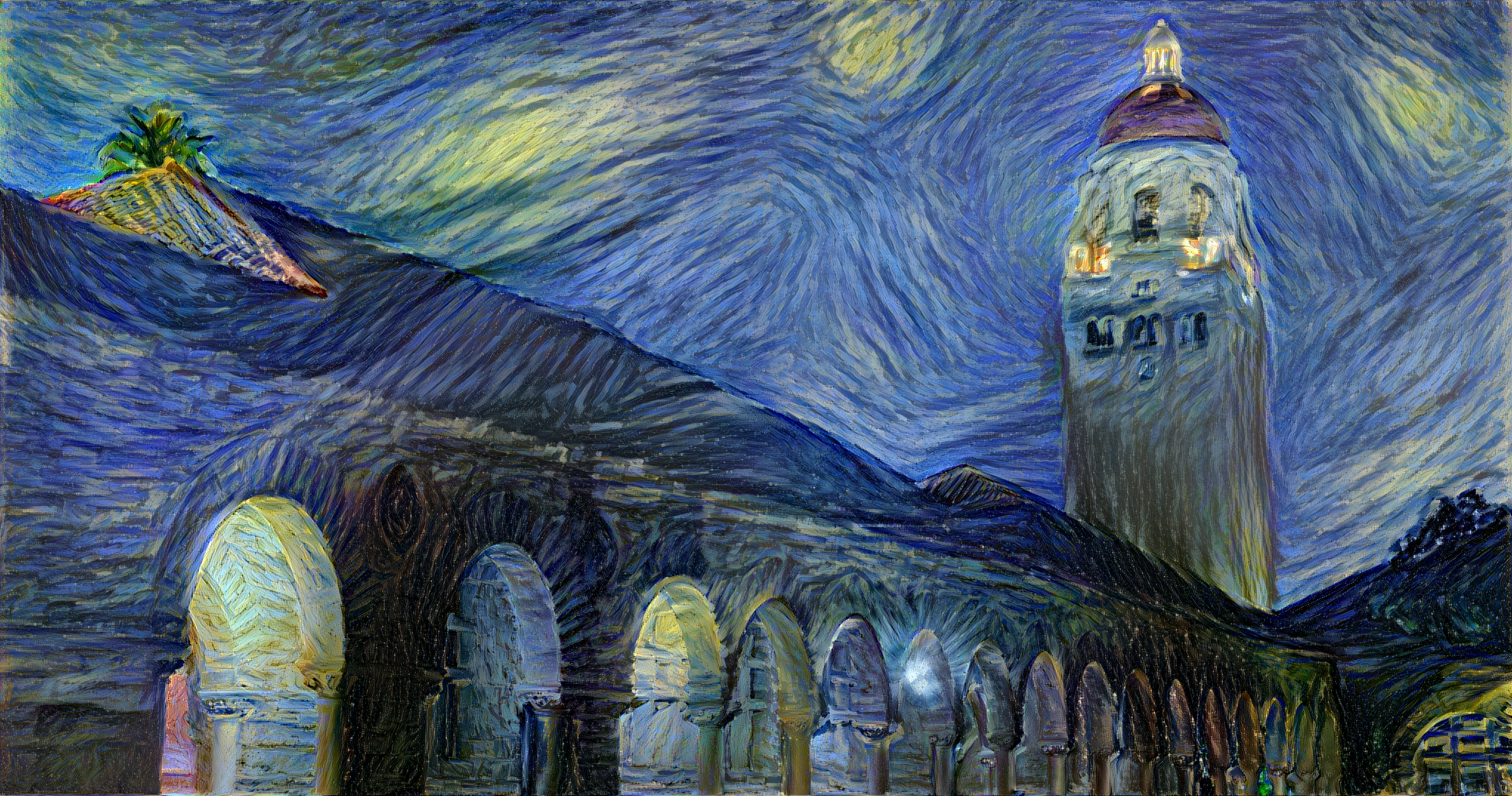
The below examples of neural style transfer are from Justin Johnson of Stanford University. The top left image is Vincent van Gogh’s The Starry Night and the top right image is a photograph of Stanford’s Hoover tower. The bottom image is generated by Justin Johnson using neural style transfer.
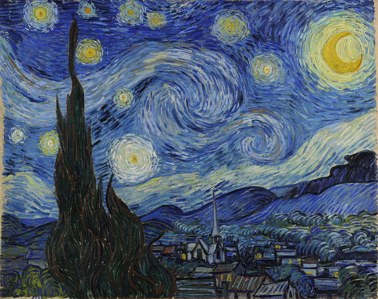

Top Left: Vincent Van Gogh’s famous artwork titled The Starry Night
Top Right: A photograph of Hoover Tower on the Stanford University campus
Bottom: A synthetic image generated by Justin Johnson that depicts Stanford University’s Hoover Tower using the style of Vincent van Gogh’s The Starry Night
History
In the 1990s, some computer science researchers began exploring non-photorealistic rendering, which offered ways to generate images inspired by the style and texture of specific artwork (such as oil paintings). However, these techniques were generally limited in the types of styles they could generate target images for.
This limitation began to disappear in 2015 with the publication of the paper A Neural Algorithm of Artistic Style. The paper’s authors demonstrated the use of convolutional neural networks to generate images inspired by many different styles.
Loss Function
Broadly, neural style transfer is the technique of using gradient descent to minimize the loss function over the following variables:
- \(x_c\) – our input content image. In the above example, this would be the photograph of Stanford University’s Hoover Tower.
- \(x_s\) – our style image. In the above example, this would be van Gogh’s The Starry Night.
- \(x\) – our generated image. In the above example, this is the generated image of Hoover Tower in the style of The Starry Night.
We intend to find a value of \(x\) that minimizes \(\alpha E_c(x, x_c) + \beta E_s(x, x_s)\) where:
- \(E_c(\cdot)\) is a function that compares the difference of content between \(x\) and \(x_c\).
- \(E_s(\cdot)\) is a function that compares the difference of style between \(x\) and \(x_s\).
- \(\alpha\) and \(\beta\) are weighting factors to balance whether the generated image favors accurate content or accurate style.
References
- neural_style: Torch implementation of neural style algorithm -- Justin Johnson
(github.com) - A Neural Algorithm of Artistic Style
(arxiv.org) - Neural Style Transfer: A Review
(arxiv.org) - Non-photorealistic rendering - Wikipedia
(en.wikipedia.org)
Neural Turing Machine (NTM)
Neural Turing Machines (NTM) consists of a RNN (commonly with LSTM), and a memory bank, where the neural network can make write and read operations. By making each operation of the NTM differentiable, it can be trained efficiently trained with gradient descent.
The main idea of the NTM is to use the memory bank – a large, addressable memory – to give a memory to the RNN so that it can read and write to, yielding a practical mechanism to learn programs. The NTM has been shown to be able to infer simple algorithms, such as copying, sorting and associative recall from input and output examples.
References
NHWC
NHWC is an acronym describing the order of the axes in a tensor containing image data samples.
Software frameworks for training machine learning models–such as TensorFlow–use the acronym NHWC
- N: Number of data samples.
- H: Image height.
- W: Image width.
- C: Image channels. A red-green-blue (RGB) image will have 3 channels.
NHWC is sometimes referred to as a channels-last layout.
Related Terms
No Free Lunch (NFL) theorem
The “No Free Lunch” theorem is the idea that all optimizers perform equally well when averaged across all possible optimization problems.
References
- Doesn't the NFL theorem show that black box optimization is flawed? - Black Box Optimization Competition
(bbcomp.ini.rub.de) - No free lunch theorem - Wikipedia
(en.wikipedia.org)
Non-max suppression
Non-max suppression refers to the idea of suppressing predicted information that is not predicted with the highest confidence.
Non-max suppression is commonly used in computer vision software, where a computer vision model may identify many nearby redundant edges or bounding boxes.
To reduce this redundancy, only the maximum feature in a set of related features are kept. For example, a computer vision model might identify a single object using multiple overlapping bounding boxes. The bounding box with the highest prediction probability is kept, and the overlapping boxes are removed in favor of the kept box. Other boxes may be unaffected by non-max suppression if they are too far away.
In the case of bounding boxes, non-max suppression is said to prune low-confidence bounding boxes that have a high intersection over union with the highest-confidence bounding box they intersect with.
References
- Non-max suppression - Computer Vision - deeplearning.ai
(www.coursera.org) - Non-maximum suppression - Computer Vision Demonstration Website
(users.ecs.soton.ac.uk)
Nonparametric clustering
Related Terms
Nonparametric regression
Related Terms
References
Nonparametric
References
Object detection
Related Terms
Object localization
Object localization is the machine learning problem that encompasses object detection–finding whether an object exists exists in an image–and finding the location of the object an image.
The location of an object in an image is typically represented as a “bounding box”.
An example of 2-dimensional object localization
Below is a rough example of what a machine learning model would output if trained and evaluated on 2D images for the purpose of drawing 2D bounding boxes around a single object. In the real world, many of the exact details may vary.
To train a machine learning model to identify the presence or absence of a single object, the model’s output would be a single 1 (for the object’s presence) or 0 (for the object’s absence). We’ll refer to this as \(p_{\mathrm{exists}}\).
But to draw a two-dimensional bounding box showing where the object is in the image, the model would need to process the image ane return a vector that looked like the following:
\[ \begin{bmatrix} p_{\mathrm{exists}} \\ b_{\mathrm x} \\ b_{\mathrm y} \\ b_{\mathrm{width}} \\ b_{\mathrm{height}} \end{bmatrix} \]
If the object exists, then the remaining values in the vector have the following meanings:
- \(b_{\mathrm x}\) is the X position of the object in the image. This may either be the center of the object, or the X position of one of the corners.
- \(b_{\mathrm y}\) is the Y position of the object in the image. This may either be the center of the object, or the Y position of one of the corners.
- \(b_{\mathrm{width}}\) is the width of the bounding box.
- \(b_{\mathrm{height}}\) is the height of the bounding box.
When the object does not exist in the given image, many machine learning models may return vectors with random numbers.
When training an object localization model, one typically uses a dataset where \(p_{\mathrm{exists}}\) is known to be 1 or 0. When evaluating an object localization model, the model typically returns \(p_{\mathrm{exists}}\) as a probability between 0 and 1. When using this probability, we may pick a threshold–such as 0.5–where we assume the model has found an object.
Different variations in object localization
In addition to 2D images from digital cameras, object localization is also relevant in other sensor data that might capture objects–such as a RADAR or LIDAR scan.
Object localization models may be trained to identify multiple objects, or to identify objects with 3D bounding boxes or non-rectangular bounding “boxes”.
Related Terms
One-dimensional convolution
One-hot encoding
One-hot encoding refers to a way of transforming data into vectors where all components are 0, except for one component with a value of 1, e,g.: \[ 0 = [1, 0, 0, 0, 0]^T \] \[ 1 = [0, 1, 0, 0, 0]^T \] \[ \ldots \] \[ 4 = [0, 0, 0, 0, 1]^T \] and so on.
One-hot encoding can make it easier for machine learning algorithms to manipulate and learn categorical variables.
References
- One-hot - Wikipedia
(en.wikipedia.org) - What is one hot encoding and when is it used in data science?
(www.quora.com)
One-shot learning
One-shot learning refers to the problem of training a statistical model (such as a classifier) with only a single example per class.
One way to build a system capable of one-shot learning is to use representation learning, to learn representations or features of data that can be used to accurately classify a single example.
Related Terms
References
Optimization
Related Terms
- 1-bit Stochastic Gradient Descent (1-bit SGD)
- Bayesian optimization
- Black-Box optimization
- Derivative-free optimization
- No Free Lunch (NFL) theorem
- Parameter budget
- Trust Region Policy Optimization (TRPO)
Out-of-core
The term out-of-core typically refers to processing data that is too large to fit into a computer’s main memory.
Typically, when a dataset fits neatly into a computer’s main memory, randomly accessing sections of data has a (relatively) small performance penalty.
When data must be stored in a medium like a large spinning hard drive or an external computer network, it becomes very expensive to randomly seek to an arbitrary section of data or to process the same data multiple times.
In such a case, an out-of-core algorithm would try to access all relevant data in one sequence.
However, modern computers have a deep memory hierarchy, and replacing random access with sequential access can increase performance even on datasets that fit within memory.
References
- Out-of-core algorithm
(en.wikipedia.org) - Scaling with instances using out-of-core learning - scikit-learn documentation
(scikit-learn.org)
Overfitting
Overfitting is when a statistical model learns patterns in the training data that are too complex to generalize well.
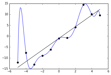
Related Terms
References
Padding (convolution)
Padding is a preprocessing step before a convolution operation.
When we convolve a \(n \times n\) image with an \(f \times f\) filter and a stride length of \(1\), the output is a matrix of dimension \(n - f \times n - f\).
For deep convolutional neural networks that may do many convolutions, this would cause the input matrix to dramatically shrink and become too small.
Additionally, values in the middle of the input matrix have a greater influence on the output than values on the edges.
There are several different methods for choosing what values to pad an input matrix with:
- Zero-padding – padding with zeroes
- Repeating the nearest border values as values for padding
- Using values from the opposite side of the matrix as padding values
Related Terms
PageRank
Related Terms
References
Paragraph vector
Paragraph Vectors is the name of the model proposed by Le and Mikolov to generate unsupervised representations of sentences, paragraphs, or entire documents without losing local word order.
This is in contrast to bag-of-words representations, which can offer useful representations of documents but lose all word order information.
Related Terms
Parameter budget
A parameter budget refers to the idea of constraining the number of learnable parameters for a machine learning model. Some types of parameters are more useful for improving a model than others, thus they should be prioritized in a model with a restricted parameter budget.
In neural networks, deeper networks seem to work better when the parameter budget is constrained.
A related idea is the computational budget, but the budget for overall computation is not strictly tied to the number of parameters in a model.
Parameter sharing
See Weight sharing.Parametric clustering
Part-of-Speech (POS) Tagging
Part-of-Speech tagging is the process of reading natural language text and assigning parts of speech to each token.
One could imagine taking in a sentence like:
The dog ran away.
and creating a data structure that had the following annotations:
The[article] dog[noun] ran[verb] away[adjective].
Words can have different parts-of-speech depending on their context. For example, the word away can be either an adverb or an adjective, or part of a larger phrase.
References
Passive-Aggressive Algorithm
References
- Online Passive-Aggressive Algorithms
(jmlr.csail.mit.edu) - Passive Aggressive Algorithms - scikit-learn Documentation
(scikit-learn.org)
PCA Color Augmentation
The term PCA Color Augmentation refers to a type of data augmentation technique first mentioned in the paper titled ImageNet Classification with Deep Convolutional Neural Networks. This paper is famous for introducing the AlexNet convolutional neural network architecture, which won the 2012 ImageNet Large Scale Visual Recognition Competition.
In general, data augmentation is the process of increasing the size of a dataset by transforming it in ways that a neural network is unlikely to learn by itself. For example, image-recognition datasets often train with images flipped vertically or horizontally.
Another form of data augmentation on image datasets is to alter the color balance of the image–for example, adjusting the values of the red, green, and blue pixels in the image.
Specifically, PCA Color Augmentation is designed to shift those values based on which values are the most present in the image. Images with heavy red values and minimal green values will have their red values altered the most through PCA Color Augmentation.
The specific mechanism relies on the principal component analysis (PCA) algorithm to find the relative color balance of a given image.
The AlexNet paper describes PCA Color Augmentation in this paragraph:
Specifically, we perform PCA on the set of RGB pixel values throughout the ImageNet training set. To each training image, we add multiples of the found principal components, with magnitudes proportional to the corresponding eigenvalues times a random variable drawn from a Gaussian with mean zero and standard deviation 0.1. Therefore to each RGB image pixel \(I_{xy} = \left [ I^R_{xy}, I^G_{xy}, I^B_{xy} \right ]^T\), we add the following quantity:
\[\left [ \mathbf p_1, \mathbf p_2, \mathbf p_3 \right ] \left [ \alpha_1 \lambda_1, \alpha_2 \lambda_2, \alpha_3 \lambda_3 \right ]^T\]
References
- ImageNet Classification with Deep Convolutional Neural Networks
(papers.nips.cc) - Fancy PCA (Data Augmentation) with Scikit-Image
(deshanadesai.github.io) - Data Augmentation - Convolutional Neural Networks - deeplearning.ai
(www.coursera.org)
Peephole connection
Peephole connections refer to a modification to the basic LSTM architecture. WildML describes LSTM peephole connections as the following:
Notably, there exist several variations on the basic LSTM architecture. A common one is creating peephole connections that allow the gates to not only depend on the previous hidden state \(s_{t-1}\), but also on the previous internal state \(c_{t-1}\), adding an additional term in the gate equations.
Peephole connections were originally introduced by Gers and Schmidhuber in 2000 to help LSTMs learn precise timings. From their abstract:
Surprisingly, LSTM augmented by “peephole connections” from its internal cells to its multiplicative gates can learn the fine distinction between sequences of spikes separated by either 50 or 49 discrete time steps.
The paper LSTM: A Search Space Odyssey gives an overview of various types of LSTM architectures and their performance, including LSTMs with peephole connections.
Perplexity
Wikipedia defines perplexity as the following:
In information theory, perplexity is a measurement of how well a probability distribution or probability model predicts a sample. It may be used to compare probability models. A low perplexity indicates the probability distribution is good at predicting the sample.
Pertainym
Pitman-Yor Topic Modeling (PYTM)
Pixel Recurrent Neural Network
References
Point Estimator
A point estimator estimates population parameters (e.g. mean, variance) with sample data.
Pointwise Mutual Information (PMI)
Related Terms
Poisson Additive Co-Clustering (PACO)
References
Policy Gradient
References
Pólya urn model
References
Polysemy
Pooling layer
A pooling layer is a common type of layer in a convolutional neural network (CNN). A pooling layer does not contain any weights that need to be learned during neural network training.
However, pooling layers come with two hyperparameters: - Stride \(s\) - Filter (or kernel) size \(f\)
Both of these hyperparameters have the same meaning as they do for convolutional layers.
Pooling layers help reduce the amount of computation a convolutional neural network needs, and can often help increase the performance of a CNN.
A pooling layer will turn an \(n \times n\) matrix into a \(\left \lfloor \frac{n - f}{s} \right ]\rfloor + 1 \times \left \lfloor \frac{n - f}{s} \right ]\rfloor + 1\) matrix.
There are several types of pooling: - Max pooling, the most common type of pooling in convolutional neural networks. - Average pooling. - Global Average Pooling (GAP). - \(k\)-Max Pooling and the closely-related Dynamic \(k\)-Max Pooling, which have found applications in neural networks for natural language processing.
Related Terms
References
Positive Pointwise Mutual Information (PPMI)
Principal Component Analysis (PCA)
Related Terms
Probabilistic Latent Semantic Indexing (PLSI)
Probabilistic Matrix Factorization (PMF)
Related Terms
Prompt engineering
Prompt engineering is the field of machine learning focused on optimizing the input prompts that are given to generative machine learning models to generate new outputs–such as text or images.
A subfield of prompt engineering is prompt injection–which focuses on the construction of malicious input prompts that can modify the behavior of a deployed generative AI system in a way unintended by its creator.
Prompt injection is analogous to other types of injection attacks in computer security, such as SQL Injection or Cross Site Scripting (XSS)
References
- Prompt Engineering -- Wikipedia
(en.wikipedia.org) - Reverse Prompt Engineering for Fun and (no) Profit
(lspace.swyx.io) - Prompt injection attacks against GPT-3 -- Simon Willison
(simonwillison.net)
Provenance tracking
In data acquisition, provenance tracking is keeping track of “where each piece of data comes from and whether it is still up-to-date”. This quoted definition comes from Philip Guo in an article for the ACM where he elaborates:
The main problem that programmers face in data acquisition is keeping track of provenance, i.e., where each piece of data comes from and whether it is still up-to-date. It is important to accurately track provenance, since data often needs to be re-acquired in the future to run updated experiments. Re-acquisition can occur either when the original data sources get updated or when researchers want to test alternate hypotheses. Also, provenance can enable downstream analysis errors to be traced back to the original data sources.
In a data science tutorial, Andrew Davison writes about the history of the term:
The term comes originally from the art world, where it refers to the chronology of the ownership and/or location of a work of art. Having detailed evidence of provenance can help to establish that a painting has not been altered or stolen, and is not a forgery. Wikipedia has a nice entry on the provenance of the Arnolfini Portrait by van Eyck. More recently, the term has been applied to other fields, including archaeology, palaeontology, and science more generally, where it refers to having knowledge of all the steps involved in producing a scientific result, such as a figure, from experiment design through acquisition of raw data, and all the subsequent steps of data selection, analysis and visualization. Such information is necessary for reproduction of a given result, and can serve to establish precedence (in case of patents, Nobel prizes, etc.)
References
- Provenance tracking - Best practices for data management in neurophysiology
(rrcns.readthedocs.io) - Data Science Workflow: Overview and Challenges - Communications of the ACM
(cacm.acm.org) - Data provenance - Wikipedia
(en.wikipedia.org)
Pseudo-labeling
Pseudo-labeling is when:
- A machine learning model is trained on a labeled training set.
- The model is used to compute predicted labels against unlabeled data.
- The model is retrained from a new dataset that adds the data with predicted labels to the training set.
Pseudo-labeling can sometimes be very effective in improving a machine learning model’s accuracy. The underlying theory is that pseudo-labeling can make it easier for a classification model to learn more precise boundaries between classes. However, in order for pseudo-labeling to work, the original training set must be large enough–and representative of all classes–for the model’s predicted labels to be reasonably accurate.
However, if the training set is already very large relative to the number of parameters in the model, then pseudo-labeling may be unnecessary.
Q-learning
R-CNN
Related Terms
References
- Rich feature hierarchies for accurate object detection and semantic segmentation
(arxiv.org) - Region Proposals - Convolutional Neural Networks - deeplearning.ai
(www.coursera.org)
Rand Index
Random Forest (RF)
Related Terms
Random initialization
Random initialization refers to the practice of using random numbers to initialize the weights of a machine learning model.
Random initialization is one way of performing symmetry breaking, which is the act of preventing all of the weights in the machine learning model from being the same.
Related Terms
References
- Why doesn't backpropagation work when you initialize the weights the same value? -- Cross Validated
(stats.stackexchange.com) - Random Initialization - Coursera Machine Learning
(www.coursera.org)
Random optimization
References
Random search
Related Terms
Receiver Operating Characteristic (ROC)
Rectified Linear Unit (ReLU)
A Rectified Linear Unit is a common name for a neuron (the “unit”) with an activation function of \(f(x) = \max(0,x)\).
Neural networks built with ReLU have the following advantages:
- gradient computation is simpler because the activation function is computationally similar than comparable activation functions like \(\tanh(x)\).
- Neural networks with ReLU are less susceptible to the vanishing gradient problem but may suffer from the dying ReLU problem.
Related Terms
References
- Why do we use ReLU in neural networks and how do we use it?
(stats.stackexchange.com) - What are the advantages of ReLU over sigmoid function in deep neural networks?
(stats.stackexchange.com)
Recurrent Neural Network Language Model (RNNLM)
A Recurrent Neural Network Language Model (RNNLM) is a recurrent neural network tasked with modeling languages.
Related Terms
References
Recurrent Neural Network
Recurrent neural networks (RNN) are feed-forward neural networks, but differently than traditional feed-forward models, RNNs contain an internal memory. A RNN have an internal loop that allows information to persist in the network. Neurons receive information not just from the previous layer, but also from themselves from the previous pass. This means that the order of inputs to the RNN matter, and may give different results with different order, as RNNs have state.
RNNs are particularly sensitive to the vanishing and exploding gradient problems, where depending on the activation functions used, the information can get lost over time. Long short-term memory networks(LSTMs) addresses this problem. RNNs are commonly used with sequential data, due to the fact that an RNN is sensitive to the order of the inputs, like in the natural language processing area. Common examples of sequential data includes texts, audio and video.
Related Terms
- Backpropagation Through Time (BPTT)
- Beam search
- Bidirectional Recurrent Neural Network (BRNN)
- Connectionist Temporal Classification (CTC)
- Gradient Clipping
- Hopfield Network
- Long Short-Term Memory (LSTM)
- Multidimensional recurrent neural network (MDRNN)
- Neural checklist model
- Neural Turing Machine (NTM)
- Pixel Recurrent Neural Network
- Recurrent Neural Network Language Model (RNNLM)
- Recursive Neural Network
- Sequence to Sequence Learning (seq2seq)
- Temporal classification
- Time-delayed neural network
References
Recursive Neural Network
Related Terms
Regression based latent factors (RLFM)
Regularization
Related Terms
REINFORCE Policy Gradient Algorithm
References
Reinforcement Learning (RL)
Reinforcement learning is about learning from feedback (reinforcement) while learning ‘on the job’, i.e. learning by trying, rather than from labeled answer data. This is how robots may learn, but is also used for playing games, a tight feedback loop through e.g. score may help give the algorithm an idea of what works well.
Related Terms
References
Reparameterization trick
References
- Auto-Encoding Variational Bayes
(arxiv.org) - How does the reparameterization trick for VAEs work and why is it important? - Cross Validated
(stats.stackexchange.com) - Variational Auto-Encoders and Extensions - NIPS 2015 workshop
(dpkingma.com)
Representation learning
Synonyms
- Feature learning
Related Terms
References
- Feature learning - Wikipedia
(en.wikipedia.org) - Representation Learning: A Review and New Perspectives
(www.cl.uni-heidelberg.de) - Representation Learning - Deep Learning Book
(www.deeplearningbook.org)
ResNet
ResNet stands for “Residual Network” and was introduced in the paper Deep Residual Learning for Image Recognition. ResNet won the ImageNet Large Scale Visual Recognition Challenge (ILSVRC) 2015 competition.
References
- Case Studies - Stanford CS231n Convolutional Neural Networks
(cs231n.github.io) - Deep Residual Learning for Image Recognition
(arxiv.org) - Identity Mappings in Deep Residual Networks
(arxiv.org)
RMSProp
Related Terms
Same convolution
A same convolution is a type of convolution where the output matrix is of the same dimension as the input matrix.
For a \(n \times n\) input matrix \(A\) and a \(f \times f\) filter matrix \(F\), the output of the convolution \(A * F\) is of dimension \(\left \lfloor \frac{n + 2p - f}{s} \right \rfloor + 1 \times \left \lfloor \frac{n + 2p - f}{s} \right \rfloor + 1\) where \(s\) represents the stride length and \(p\) represents the padding.
In a same convolution:
- \(s\) is typically set to \(1\)
- \(p\) is set to \(\frac{f - 1}{2}\)
- \(f\) is an odd number
The result is that \(A\) is padded to be \(n + p \times n + p\) and \(A * F\) becomes \(n \times n\) – the same as the original dimensions of \(A\).
Related Terms
References
Search-based software engineering (SBSE)
Search-based software engineering applies search and optimization techniques to software engineering problems.
[LDADE][/terms/latent-dirichlet-allocation-differential-evolution-ldade] is an example of a system that applies search-based software engineering to optimize topic modeling.
Related Terms
References
Second-order information
The term second-order information refers to information about a function gained by computing its second derivative. The second derivative reveals information about the function’s curvature.
Self-supervised learning
Self-supervised learning is a type of supervised learning where the training labels are determined by the input data.
word2vec and similar word embeddings are a good example of self-supervised learning. word2vec models predict a word from its surrounding words (and vice versa). Unlike “traditional” supervised learning, the class labels are not separate from the input data.
Autoencoders are another example of self-supervised learning, as they are trained to shrink and reconstruct their inputs.
Related Terms
References
- Is there any difference between distant supervision, self-training, self-supervised learning, and weak supervision? - Cross validated
(stats.stackexchange.com) - Self-supervised learning - Virginia R. de Sa
(www.cogsci.ucsd.edu)
Semantic hashing
A hash is a small, lossy representation of a data point. Typically hashes are fixed-sized representations of variable-sized data.
Cryptographic hash functions take and data and return fixed-size representations. These typically have the property that the hash value (ideally) reveals no information about the original piece of data.
The MD5 hash for the string hello is 5d41402abc4b2a76b9719d911017c592, but the hash for Hello is 8b1a9953c4611296a827abf8c47804d7. It is typically not trivial to infer that these two distinct-looking hashes have similar inputs.
Semantic hashes are the opposite – they are fixed-length representations where similar pieces of input data should have similar hashes. Word embeddings are a type of semantic hash for words. Words that occur in contexts end up with similar embeddings.
Semantic hashes are useful for document search, information retrieval, or other problems where one needs to find similar pieces of data.
References
Semi-supervised learning
Semi-supervised learning mixes labeled and labeled data to produce better models.
In machine learning, finding or creating correctly-labeled data (e.g. images with annotations and descriptions, audio with text transcriptions) can be difficult or expensive.
Semi-supervised learning techniques take advantage of a small amount of labeled data and a large amount of unlabeled data to produce a better model than a purely supervised learning or a purely unsupervised learning technique.
Related Terms
References
- Is there any difference between distant supervision, self-training, self-supervised learning, and weak supervision? - Cross validated
(stats.stackexchange.com) - Self-supervised learning - Virginia R. de Sa
(www.cogsci.ucsd.edu) - Semi-supervised learning - Wikipedia
(en.wikipedia.org)
sense2vec
sense2vec refers to a system in a paper titled sense2vec - A Fast and Accurate Method for Word Sense Disambiguation In Neural Word Embeddings. It solves a problem with previous word embeddings like word2vec and GloVe where words of different senses (e.g. “duck” as an animal and “duck” as a verb) are represented by the same embedding.
sense2vec uses word sense information to train more accurate word embeddings.
References
- sense2vec - A Fast and Accurate Method for Word Sense Disambiguation In Neural Word Embeddings
(arxiv.org) - Sense2vec with spaCy and Gensim - Explosion AI
(explosion.ai)
Sequence to Sequence Learning (seq2seq)
This typically refers to the method originally described by Sutskever et al. in the paper Sequence to Sequence Learning with Neural Networks.
Feedforward neural networks and many other models can learn complex patterns, but require fixed-length input. This makes it difficult for these models to learn variable-length sequences. To solve this, the authors applied one LSTM to read the input seqeunce and a second LSTM to generate the output sequence.
A few potential applications of sequence to sequence learning include:
- Machine translation
- Text summarization
- Speech-to-text conversion
Related Terms
References
- Sequence-to-Sequence Models - TensorFlow Tutorials
(www.tensorflow.org) - Sequence to Sequence Learning with Neural Networks
(arxiv.org)
Sequential Model-Based Optimization (SMBO)
References
Sequential pattern mining
References
Siamese neural network
A Siamese neural network is a neural network architecture that runs two pieces of data through identical neural networks, and then the outputs are fed to a loss function measuring similarity between outputs.
Siamese neural networks are a common model architecture for one-shot learning.
For example, a Siamese neural network might be used to train a model to measure similarity between two different images, for the purpose of identifying whether the images are of the object…. but without training on many examples of that object.
References
Similarity learning
Similarity learning is the area of machine learning focusing on learning how similar or different two objects are.
Similarity learning is often used in areas of machine learning where there are not a fixed number of classes that objects fit into. Face verification is one example of such an area.
Learning-to-rank is another area of machine learning where the model needs to learn a similarity function between the pieces of data in the dataset.
Distance metric learning is related to similarity learning, but where the similarity function is also required to obey the four axioms of a distance metric. Outside of distance metric learning, similarity learning often learns a pseudometric, where not all four axioms of a distance metric are true.
Related Terms
References
Singular Value Decomposition (SVD)
Related Terms
Skip-Gram
Related Terms
Smooth support vector machine (SSVM)
References
Sobel filter (convolution)
The Sobel filter is a set of two convolution filters used to detect horizontal and vertical edges in images.
The horizontal filter is
\[ \begin{bmatrix} 1 & 0 & -1 \\ 2 & 0 & -2 \\ 1 & 0 & -1 \end{bmatrix} \]
and the vertical filter is
\[ \begin{bmatrix} 1 & 2 & 1 \\ 0 & 0 & 0 \\ -1 & -2 & -1 \end{bmatrix} \]
References
Softmax
The softmax turns \(n\) numbers in \(\mathbb R^N\) into a probability distribution proportional to the size of the numbers.
Given an \(n\)-dimensional vector \(\mathbf v\) with all component terms in \(\mathbb R^N\), the softmax of \(\mathbb v\) is: \[ \mathrm{softmax}(\mathbb v)_i = \frac{\exp{(v_i)}} {\sum_{j=1}^{n} \exp{(v_i)}} \]
References
Sparse autoencoder
Spearman's Rank Correlation Coefficient
Stacked autoencoder
Standard deviation
References
Stationary environment
A stationary environment refers to data-generating distributions that do not change over time.
A non-stationary environment, in contrast, refers to data-generating distributions that do change over time.
It is a difficult problem to train machine learning algorithms to generalize well in non-stationary environments. See Machine Learning in Non-Stationary Environments for more information.
Stochastic block model (SBM)
The stochastic block model is a common model for detection of community structure
Related Terms
Stochastic convex hull (SCH)
References
- On the expected diameter, width, and complexity of a stochastic convex-hull
(arxiv.org) - On the Separability of Stochastic Geometric Objects, with Applications
(arxiv.org) - Convex Hulls under Uncertainty
(www.cs.ucsb.edu) - Probabilistic Convex Hull Queries over Uncertain Data
(ieeexplore.ieee.org)
Stochastic Gradient Descent (SGD)
Related Terms
- 1-bit Stochastic Gradient Descent (1-bit SGD)
- ADADELTA
- AdaGrad
- ADAM Optimizer
- Learning rate decay
- Minibatch Gradient Descent
- Momentum
- Prompt engineering
Stochastic Gradient Variational Bayes (SGVB)
Stochastic Optimization
Related Terms
Stride (convolution)
In convolutions, the stride is the number of horizontal and vertical steps that the filter takes over the original matrix.
Structured Bayesian optimization (SBO)
Related Terms
References
Structured learning
Related Terms
References
- Structured prediction - Wikipedia
(en.wikipedia.org) - What is structured learning? - PyStruct
(pystruct.github.io)
Supervised learning
Supervised learning is about training on labeled data, i.e. questions with known answers. The task is to find the function that maps a set of inputs (x1, x2, x3, …) to the value to be predicted (y).
Related Terms
- Bias-variance tradeoff
- Distance metric learning
- Overfitting
- Reinforcement Learning (RL)
- Self-supervised learning
- Semi-supervised learning
- Similarity learning
- Transduction
- Unsupervised learning
References
Support Vector Machine (SVM)
Support Vector Machine is a classification method in supervised learning that seeks to use support vectors (cases close to the boundary) to find an optimal hyperplane separating items from different classes.
Related Terms
Symmetry breaking
Symmetry breaking refer to a requirement of initializing machine learning models like neural networks.
When some machine learning models have weights all initialized to the same value, it can be difficult or impossible for the weights to differ as the model is trained. This is the “symmetry”.
Initializing the model to small random values breaks the symmetry and allows different weights to learn independently of each other.
Related Terms
References
- Why doesn't backpropagation work when you initialize the weights the same value? -- Cross Validated
(stats.stackexchange.com) - Random Initialization - Coursera Machine Learning
(www.coursera.org)
Synset
A synset is WordNet’s terminology for a synonym ring.
WordNet is a database of English words grouped into sets of synonyms. WordNet’s synsets are often useful in information retrieval and natural langauge processing tasks to discover when two different words can mean similar things.
SyntaxNet
SyntaxNet is a framework for natural language syntactic parsers released by Google in 2016.
SyntaxNet tags words in a sentence with their syntactic part-of-speech and creates a parse tree showing dependencies between words in a sentence.
Parsey McParseface is a SyntaxNet model trained on the English language. At its time of release, Parsey McParseface is the world’s most accurate model of its kind.
References
- Announcing SyntaxNet: The World’s Most Accurate Parser Goes Open Source - Google Research Blog
(research.googleblog.com) - Globally Normalized Transition-Based Neural Networks
(arxiv.org)
Tabu Search
References
- Tabu Search - Clever Algorithms
(www.cleveralgorithms.com) - Tabu search - Wikipedia
(en.wikipedia.org)
Temporal classification
Related Terms
Temporal Generative Adversarial Network (TGAN)
References
Termite
Termite is a visual analysis tool to determine the quality of topic models like latent Dirichlet allocation.
Termite lays out document terms as a table of circles where:
- rows represent document terms
- columns represent topics
- circular areas represent term probabilities
References
- Termite: Visualization Techniques for Assessing Textual Topic Models - Stanford Visualization Group
(vis.stanford.edu) - Online Termite Demo
(vis.stanford.edu) - Termite Data Server - Github
(github.com)
Test term
This is the body of yet another test term. I think that this is going to be extremely promising.
$$
_0^100 x^2
$$
TextRank
TextRank is a graph ranking algorithm applied to text. It is useful for various unsupervised learning tasks in natural language processing.
Related Terms
References
Textual entailment
See Entailment.Time-delayed neural network
Time-delayed signal
Top-1 error rate
The term top-1 error rate refers method of benchmarking machine learning models in the ImageNet Large Scale Visual Recognition Competition.
The model is considered to have classified a given image correctly if the target label is the model’s top prediction. This is in contrast to the top-5 error rate where the model only needs to identify the correct label in the model’s top 5 predictions.
Related Terms
References
Top-5 error rate
The term top-5 error rate refers method of benchmarking machine learning models in the ImageNet Large Scale Visual Recognition Competition.
The model is considered to have classified a given image correctly if the target label is one of the model’s top 5 predictions.
References
Training, validation, and test datasets
When a labeled dataset is used to train machine learning models, it is common to break up the dataset into three parts:
- Training: used to directly improve the model’s parameters.
- Validation: used to evaluate a model’s performance while optimizing the model’s hyperparameters.
- Test: used to evaluate a model after hyperparameter optimization is complete.
Why the validation and test datasets are necessary
During the process of training a machine learning model, it is common for a model’s parameters to overfit to the training dataset. These models report artificially high accuracy against the training dataset, but they perform poorly against data not in the training dataset.
To realistically measure a model’s performance, it is better to evaluate it against a validation dataset that was not used when training the model.
You can train multiple models with different hyperparameters and compare them with the same validation dataset. But this creates a new problem: just like a model’s parameters can overfit to the training dataset, a model’s parameters and hyperparameters can overfit to the validation dataset.
To realistically measure a set of models, it is better to evaluate them against a test dataset not used for training or validation. The test dataset is used to measure the performance of your various models at the end of the training process. Be careful not to repeatedly use the test dataset to re-train models or choose models, otherwise you risk creating models that have overfit to the test dataset.
Picking the size of the validation and test datasets
The validation and test datasets need to be larger than a certain minimum size. Otherwise, the model’s validation and test accuracy will not be representative of the “real-world” acccuracy. If your input dataset is very small, you can use cross-validation to train and evaluate a model against many different training/validation/test splits.
For medium-sized datasets, it is typical for the validation and test datasets to each be 10%-30% of the total amount of data. For example, a common training/validation/test split is 60%/20%/20%.
However, the validation and test datasets do not need to be larger than a certain absolute size. Above that size, adding more validation or test data does not make the model’s performance metrics more realistic. If your input dataset contains millions of data samples, then you may only need about 1% each for the validation and test datasets.
How to balance the validation and test datasets
Preserve imbalanced classes
If you are working on a classification problem with imbalanced classes–such as a dataset where one class is 99% of the dataset and the other class is 1% of the dataset–then you might consider improving the training process by oversampling the smaller class. But for your validation and test datasets, you want to measure your model’s performance against the same class balance that your model would encounter in the real world.
Validation and test datasets should have “newer” samples
If you are training a model on time series data, typically your goal is to predict something about the future using data from the past or present.
In order to properly evaluate a time series model, your training/validation/test split must obey the “arrow of time”:
- All of the data samples in your validation dataset should be newer than your training dataset.
- All of the data samples in your test dataset should be newer than your validation dataset.
If your training dataset contains data samples that are newer than your validation dataset, then your model’s validation accuracy will be misleadingly high. Your model is effectively traveling backward in time if it trains on new data and evaluates on old data.
Many people make the mistake of randomly shuffling the input dataset before splitting it into a training, validation, and test datasets–effectively violating the arrow of time.
Do not apply data augmentation
Data augmentation is the use of computer algorithms to create or modify training data samples. The goal of data augmentation is to increase the size of the training dataset and to act as a regularizer–something that reduces a model’s ability to overfit.
However, when a machine learning model is deployed to the “real world” and is making predictions, typically the model will not perform any augmentation or regularization on its input. To mirror the real world, a model should not perform augmentation or regularization on the validation or test dataset.
There are a few exceptions to the rule:
- If the validation and/or test datasets are too small for a model to reliably evaluate, then it might make sense to use data augmentation to add data samples.
- If the entire training dataset is computer-generated–like a dataset of images generated from a video game–then it may be reasonable for the validation and test datasets to also be entirely computer-generated.
References
Transduction
Similar to supervised learning, but does not explicitly construct a function: instead, tries to predict new outputs based on training inputs, training outputs, and new inputs.
References
Tree-LSTM
Tree-LSTMs are a variant of Long Short Term Memory (LSTM) neural networks.
A traditional LSTM is structured as a linear chain, and displays strong performance on sequence modeling tasks–such as machine translation.
However, some types of data (such as text) are better represented as tree structures instead of sequences. Thus, Tree-LSTMs were introduced by Tai, et al in 2015.
Related Terms
References
Triplet loss function
See Triplet loss.Triplet loss
Triplet loss is a loss function that come from the paper FaceNet: A Unified Embedding for Face Recognition and Clustering. The loss function is designed to optimize a neural network that produces embeddings used for comparison.
The loss function operates on triplets, which are three examples from the dataset:
- \(x_i^a\) – an anchor example. In the context of FaceNet, \(x_i^a\) is a photograph of a person’s face.
- \(x_i^p\) – a positive example that has the same identity as the anchor. In FaceNet, this is a second picture of the same person as the picture from the anchor example.
- \(x_i^n\) – a negative example that represents a different entity. For FaceNet, this would be an image of a second person–someone different than the person represented by the anchor and positive examples.
The triplet loss function is designed to train the model to produce embeddings such that the positive example \(x_i^p\) is closer to the anchor than the negative example \(x_i^n\).
Math Details
More formally, for an embedding function \(f(x) \in \mathbb R^d\) that embeds input data \(x\) into a \(d\)-dimensional vector, we want
\[ ||f(x_i^a) - f(x_i^p)||_2^2 + \alpha \leq ||f(x_i^a) - f(x_i^n)||_2^2 \]
for all \(N\) possible triplets of \(x_i^a\), \(x_i^p\), and \(x_i^n\). The \(||x||_2^2\) operator is the square of the Eucledian norm. The \(\alpha\) symbol stands for a margin to ensure that the model doesn’t make the embeddings \(f(x_i^a)\), \(f(x_i^p)\), and \(f(x_i^n)\) equal each other to trivially satisfy the above inequality.
This leads to the following loss function over the \(N\) possible triplets.
\[ \sum_i^N \left [ ||f(x_i^a) - f(x_i^p)||_2^2 - ||f(x_i^a) - f(x_i^n)||_2^2 + \alpha \right ]_+ \]
the \([x]_+\) operator stands for \(\max(0,x)\).
Triplet selection
In a typical dataset, many triplets of \(x_i^a\), \(x_i^p\), and \(x_i^n\) will satisfy the inequality in the previous section without the algorithm learning a useful embedding. This slows down the training of a machine learning algorithm that uses the triplet loss function.
To speed training back up, it makes sense to train the algorithm on examples where \(f(x_i^a)\) is closer to \(f(x_i^n)\) than \(f(x_i^p)\) in the embedding space (ignoring the term \(\alpha\)).
Synonyms
- Triplet loss function
Related Terms
References
- Triplet Loss - Convolutional Neural Networks - deeplearning.ai
(www.coursera.org) - In Defense of the Triplet Loss for Person Re-Identification
(arxiv.org) - FaceNet: A Unified Embedding for Face Recognition and Clustering
(arxiv.org)
Troponym
Trust Region Policy Optimization (TRPO)
Related Terms
References
Underfitting
Related Terms
UNK
UNK, unk, <unk> are variants of a symbol in natural language processing and machine translation to indicate an out-of-vocabulary word.
Many language models do calculations upon representations of the \(n\) most frequent words in the corpus. Words that are less frequent are replaced with the <unk> symbol.
This is what such a transformation might look like. The below is an example of a source document in a corpus with common English words.
Today I’ll bake; tomorrow I’ll brew, Then I’ll fetch the queen’s new child, It is good that no one knows, Rumpelstiltskin is my name.
Every word in the above quote is common in English, except for Rumpelstiltskin, which is replaced as following:
Today I’ll bake; tomorrow I’ll brew, Then I’ll fetch the queen’s new child, It is good that no one knows, <unk> is my name.
Unsupervised learning
Unsupervised learning is about problems where we don’t have labeled answers, such as clustering, dimensionality reduction, and anomaly detection.
Related Terms
- Dimensionality reduction
- Distance metric learning
- Reinforcement Learning (RL)
- Self-supervised learning
- Semi-supervised learning
- Similarity learning
- Supervised learning
References
Valid convolution
A valid convolution is a type of convolution operation that does not use any padding on the input.
For an \(n \times n\) input matrix and an \(f \times f\) filter, a valid convolution will return an output matrix of dimensions
\[ \left \lfloor \frac{n - f}{s} + 1 \right \rfloor \times \left \lfloor \frac{n - f}{s} + 1 \right \rfloor \]
where \(s\) is the stride length of the convolution.
This is in contrast to a same convolution, which pads the \(n \times n\) input matrix such that the output matrix is also \(n \times n\).
References
Vanishing gradient problem
Variance
Wikipedia describes variance as follows:
In probability theory and statistics, variance is the expectation of the squared deviation of a random variable from its mean, and it informally measures how far a set of (random) numbers are spread out from their mean.
Variance the square of standard deviation, or rather, standard deviation is the square root of variance. Thus, sometimes variance is written as \(\sigma^2\) where \(\sigma\) stands for the standard deviation.
Related Terms
References
Variation of Information distance
Related Terms
References
Variational Autoencoder (VAE)
Related Terms
- Adversarial autoencoder
- Adversarial Variational Bayes
- Codebook
- Reparameterization trick
- Vector-Quantized Variational Autoencoders (VQ-VAE)
Vector-Quantized Variational Autoencoders (VQ-VAE)
The Vector-Quantized Variational Autoencoder (VAE) is a type of variational autoencoder where the autoencoder’s encoder neural network emits discrete–not continuous–values by mapping the encoder’s embedding values to a fixed number of codebook values.
The VQ-VAE was originally introduced in the Neural Discrete Representation Learning paper from Google.
Related Terms
References
- Understanding VQ-VAE (DALL-E Explained Pt. 1) - Machine Learning @ Berkeley
(ml.berkeley.edu) - Neural Discrete Representation Learning
(arxiv.org)
VGGNet
VGGNet is a deep convolutional neural network for image recognition, trained by the Visual Geometry Group (VGG) at the University of Oxford.
VGGNet helped the VGG team secure the first place in Localization and second place in Classification in the 2014 ImageNet Large Scale Visual Recognition Competition.
Related Terms
References
- Very Deep Convolutional Networks for Large-Scale Visual Recognition - Department of Engineering Science, University of Oxford
(www.robots.ox.ac.uk) - Case Studies - Stanford CS231n Convolutional Neural Networks
(cs231n.github.io) - Very Deep Convolutional Networks for Large-Scale Image Recognition
(arxiv.org)
Weak supervision
Weak supervision describes the use of noisy or error-prone data labels for training supervised learning models.
It can be expensive or impractical to create or obtain highly-accurate labels for a large dataset. Weak supervision offers the choice of using a larger number of somewhat-less-accurate data labels.
References
- Weak Supervision: A New Programming Paradigm for Machine Learning - The Stanford AI Lab Blog
(ai.stanford.edu) - Snorkel and The Dawn of Weakly Supervised Machine Learning - Stanford DAWN
(dawn.cs.stanford.edu) - Snuba: Automating Weak Supervision to Label Training Data - Stanford University
(www.vldb.org) - Weak supervision - Wikipedia
(en.wikipedia.org)
Weight sharing
In neural networks, weight sharing is a way to reduce the number of parameters while allowing for more robust feature detection. Reducing the number of parameters can be considered a form of model compression.
Synonyms
- Parameter sharing
References
- Simplifying Neural Networks by Soft Weight-Sharing
(www.cs.toronto.edu) - Shared Weights - Convolutional Neural Networks - Deep Learning Tutorial
(deeplearning.net) - Soft Weight-Sharing for Neural Network Compression
(arxiv.org)
Weighted finite-state transducer (WFST)
References
Wide convolution
Word embedding
A word embedding (or word vector) refers to a dense vector representation of a word.
Before word embeddings, words were typically represented with sparse vectors in bag-of-words models or with n-grams.
Word embeddings are typically trained with an unsupervised model over a large corpus of text. In the training process, the vectors are updated to better predict elements of the corpus, such as words surround a given target word.
At the end of this process, word embeddings often have geometric relations to each other that encode semantic meaning. A common example for this is using vector addition and subtraction to find related words. The vector \(\mathrm{King}_v - \mathrm{Man}_v + \mathrm{Woman}\) is most similar to the vector \(\mathrm{Queen}_v\). This example comes from the project page for word2vec.
Common implementations of word embeddings include:
Related Terms
- Continuous-Bag-of-Words (CBOW)
- Distributed representation
- Embed, Encode, Attend, Predict
- fastText
- GloVe (Global Vectors) embeddings
- Self-supervised learning
- Semantic hashing
- sense2vec
- Skip-Gram
- word2vec
word2phrase
word2phrase refers to a program in the word2vec toolkit that discovers multi-word phrases in a corpus of words.
From the original word2vec Google Code page:
In certain applications, it is useful to have vector representation of larger pieces of text. For example, it is desirable to have only one vector for representing ‘san francisco’. This can be achieved by pre-processing the training data set to form the phrases using the word2phrase tool, as is shown in the example script ./demo-phrases.sh.
word2vec
word2vec refers to a pair of models, open-source software, and pre-trained word embeddings from Google.
The models are:
- skip-gram, using a word to predict the surrounding \(n\) words
- continuous-bag-of-words (CBOW), using the context of the surrounding \(n\) words to predict the center word.
The original paper is titled Efficient Estimation of Word Representations in Vector Space by Mikolov et al.
The source code was originally hosted on Google Code but is now located on Github.
Related Terms
- Continuous-Bag-of-Words (CBOW)
- fastText
- GloVe (Global Vectors) embeddings
- Self-supervised learning
- sense2vec
- word2phrase
References
- Efficient Estimation of Word Representations in Vector Space
(arxiv.org) - Vector Representations of Words - Tutorials - TensorFlow Documentation
(www.tensorflow.org)
Wronskian matrix
Related Terms
YOLO (object detection algorithm)
YOLO (an acronym standing for the phrase “You Only Look Once”) refers to a fast object detection algorithm. Previous attempts at building object detection algorithms involved running object detectors or object localizers multiple times over a single image.
Instead of needing multiple executions over a single image, YOLO detects objects through sending an image through a single forward pass through a convolutional neural network.
Related Terms
References
YOLO9000 (object detection algorithm)
See YOLOv2 (object detection algorithm).YOLOv2 (object detection algorithm)
Synonyms
- YOLO9000 (object detection algorithm)
References
Zero padding
Signal processing
In signal processing, zero padding refers to the practice of adding zeroes to a time-domain signal. Zero-padding is often done before performing a fast Fourier transform on the time-domain signal.
Neural networks
In convolutional neural networks, zero-padding refers to surrounding a matrix with zeroes. This can help preserve features that exist at the edges of the original matrix and control the size of the output feature map.
Below is an example of a padding operator \(\mathrm{Pad}(n, \mathbf X)\) that adds \(n\) layers of zeroes around the matrix \(\mathbf X\). \[ \mathbf X = \begin{bmatrix} a & b & c \\ d & f & g \\ h & j & k \end{bmatrix}, \] \[ \mathrm{Pad}(1, \mathbf X) = \begin{bmatrix} 0 & 0 & 0 & 0 & 0 \\ 0 & a & b & c & 0 \\ 0 & d & f & g & 0 \\ 0 & h & j & k & 0 \\ 0 & 0 & 0 & 0 & 0 \end{bmatrix} \]
Related Terms
References
- FFT Zero Padding - Bitweenie
(www.bitweenie.com) - Why should I zero-pad a signal before taking the Fourier transform? - Statistics StackExchange
(dsp.stackexchange.com) - Convolutional Layers: To pad or not to pad?
(stats.stackexchange.com)
Zero-shot learning
Ian Goodfellow in a Quora answer defines zero-shot learning as the following:
Zero-shot learning is being able to solve a task despite not having received any training examples of that task. For a concrete example, imagine recognizing a category of object in photos without ever having seen a photo of that kind of object before. If you’ve read a very detailed description of a cat, you might be able to tell what a cat is in a photograph the first time you see it.
Related Terms
References
- What is zero-shot learning?
(www.quora.com) - Representation Learning - Deep Learning Book
(www.deeplearningbook.org)